tcPDA
Contents
tcPDA (three-color photon distribution analysis) is the module for quantitative analysis of three-color FRET data to extract the underlying distance distributions, similar to the PDAFit module for two-color FRET data. It implements the algorithms described in [Barth2018].
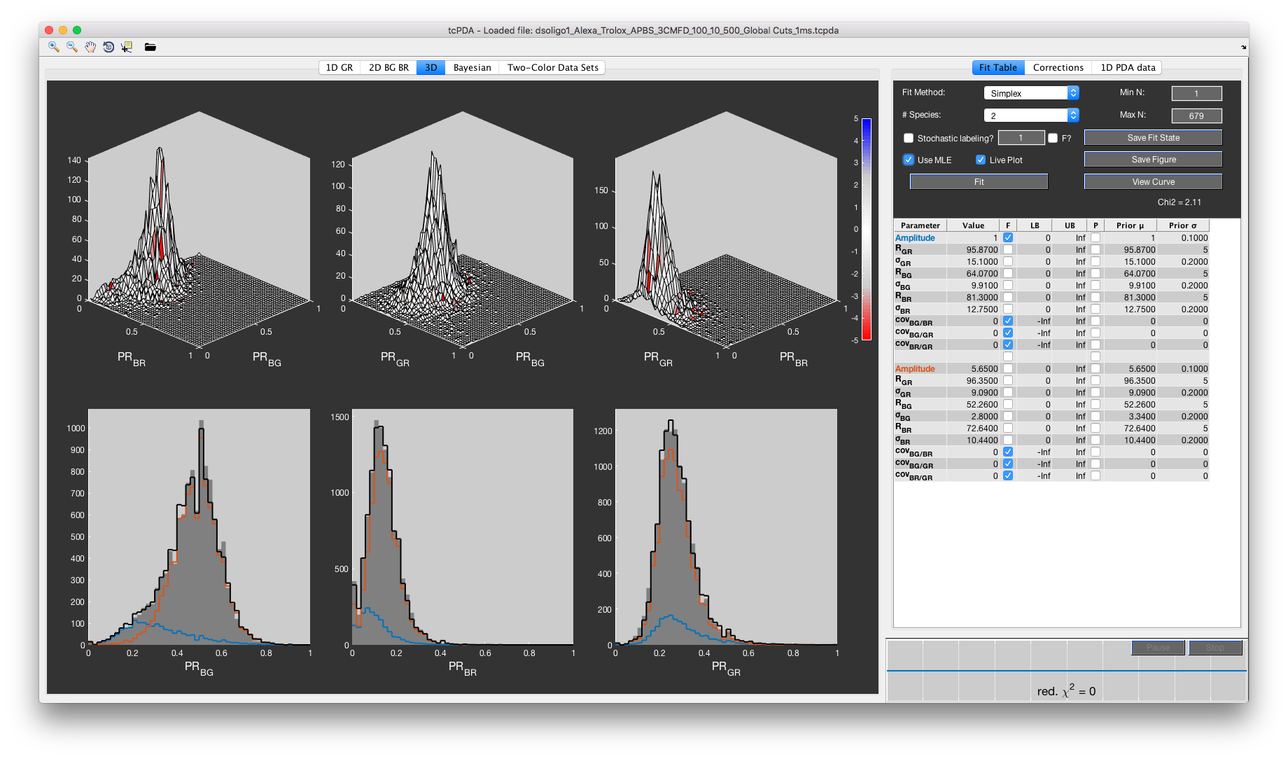
The main GUI of tcPDA
Data loading
From BurstBrowser
To process and export burst data from the BurstBrowser module to tcPDA, use the PDA export functionality in BurstBrowser. Load data (.tcpda files) by clicking on the folder icon in the top left.
From text file
As an alternative to the MATLAB-based .tcpda file format, it is also possible to load text-based data into the tcPDA program. The text-based file format is a comma-separated file containing the time bin size in milliseconds and a list of the photon counts per time bin for all detection channels \(N_{BB}, N_{BG}, N_{BR}, N_{GG}, N_{GR}\).
The basic structure of the text-based file format with ending .txt is given by the following template.
# place for comments
timebin = 1; # timebin in ms
NBB, NBG, NBR, NGG, NGR
46,54,16,95,28
35,60,17,113,46
38,58,14,82,33
67,51,10,94,23
20,32,6,36,13
32,35,9,46,23
7,37,20,50,14
...
...
As before, load it using the folder icon in the top left, and select “Text-based tcPDA file” in the file dialog.
Fitting data
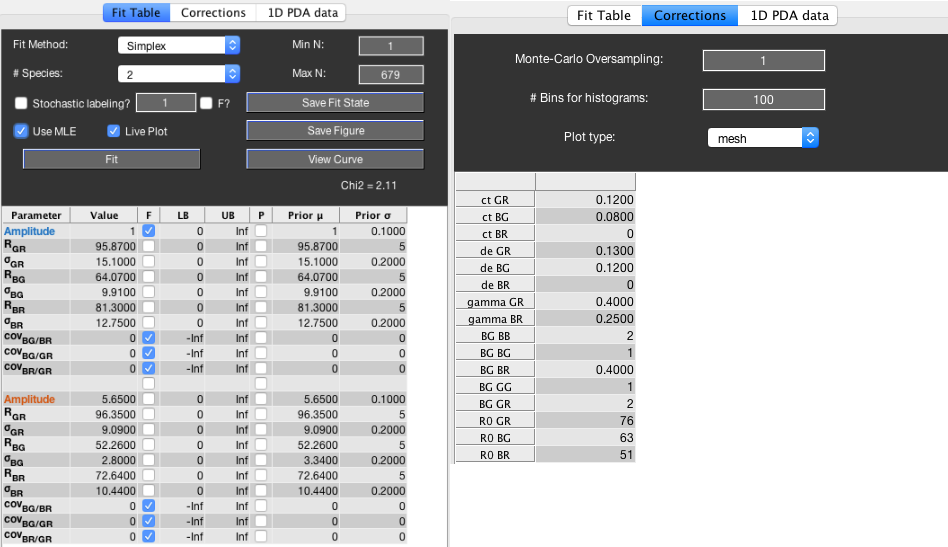
Left: The Fit Table tab contains options for the fit routine and model functions. Right: The Corrections tab allows to set the correction factors.
Defining the correction factors
The correction factors can be set in the Corrections tab. If data has been exported from the BurstBrowser module, the values for crosstalk (ct), gamma-factors (gamma), Förster radii (R0) and background counts in kHz (BG) will be automatically transferred to tcPDA and need not be set. However, the value for the direct excitation probabilities (de) is different in tcPDA compared to the intensity-based corrections to photon counts in BurstBrowser (see also the respective section in the manual for PDAFit). The direct excitation probability of dye \(X\) after excitation by laser \(Y\), where \(X,Y \in \{B,G,R\}\), is denoted by \(p_{de}^{XY}\) (called de in the GUI). It is defined based on the extinction coefficients \(\varepsilon_X^{\lambda_Y}\):
The other parameters in the Corrections tab are explained in the further sections.
The fit parameter table
The fit parameter table allows to set the initial values for the parameters. It adapts to the selected number of species, whereby the color of the Amplitude parameter indicates the color of the species in the plots. Check the F option to fix parameters. Lower and upper boundaries (LB and UB) are by default set to 0 and infinity, but can be specified if needed. The other columns are related to the usage of prior information and are described in the respective section.
Note
The amplitudes are normalized by the fit routine, i.e. \(\sum_i A_i = 1\). To reduce the number of free fit parameters, the amplitude of the first species is fixed by default, but can be unfixed by the user.
Performing the fit
Start the fit by clicking the Fit button in the Fit Table tab. The fit options are described in detail here. To simply view the theoretical histograms of the current model, click the View Curve button.
It is usually best to perform the fit of the three-color FRET histogram in three steps of increasing complexity. Since alternating excitation of the blue, green and red lasers is employed, the direct excitation of the green dye is essentially equivalent to performing a two-color FRET experiment, which can be fit first (1D GR tab). Then, one can fit the distribution of the proximity ratios BG and BR while keeping the center value and standard deviation for the distance \(R_{GR}\) fixed (2D BG BR tab). Finally, the full three-dimensional distribution of the proximity ratio GR, BG and BR can be fit by setting all parameters free (3D tab).
The following sections describe the individual steps. The Fit Table tab applies to all three tabs (1D GR, 2D BG BR and 3D) in the main window and adapts functionality based on which main window is selected.
Fitting the histogram of proximity ratio GR
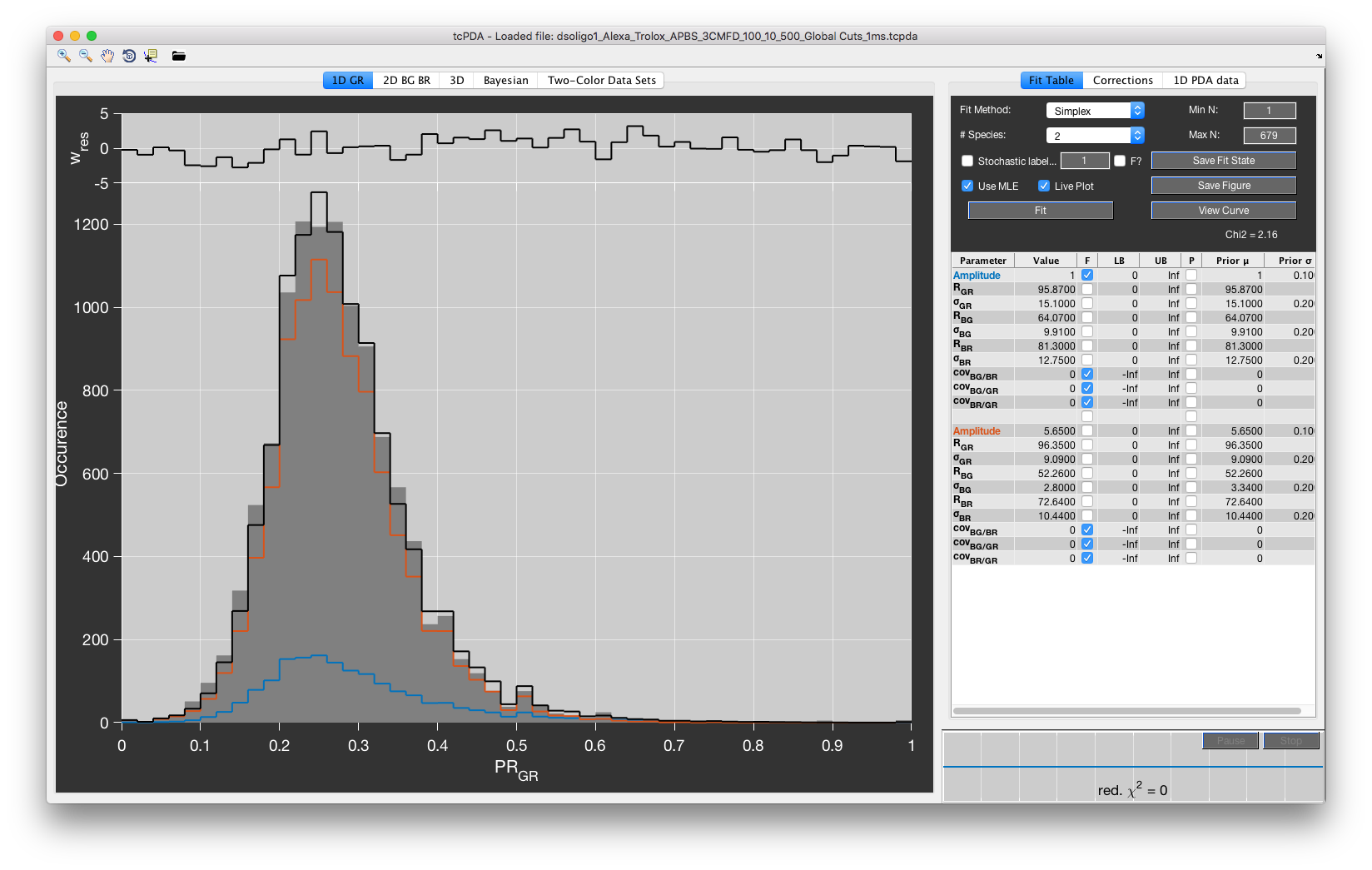
Fitting the one-dimensional histogram of the proximity ratio GR.
The 1D GR tab allows fitting of the one-dimensional distribution of the proximity ratio GR, disregarding the available three-color information. It is useful to pre-fit the values for \(R_{GR}\) and \(\sigma_{GR}\) and get a first idea of the number of populations required to describe the data. Only the amplitudes and parameters \(R_{GR}\) and \(\sigma_{GR}\) are fit. Fitting of the one-dimensional histogram of proximity ratio GR is always performed using Monte Carlo simulation of the histogram with the Simplex fit algorithm, regardless of the fit options set in the Fit Table tab. The settings Use MLE, Stochastic Labeling and Fit Method thus have no effect.
Fitting the two-dimensional histogram of proximity ratios BG and BR
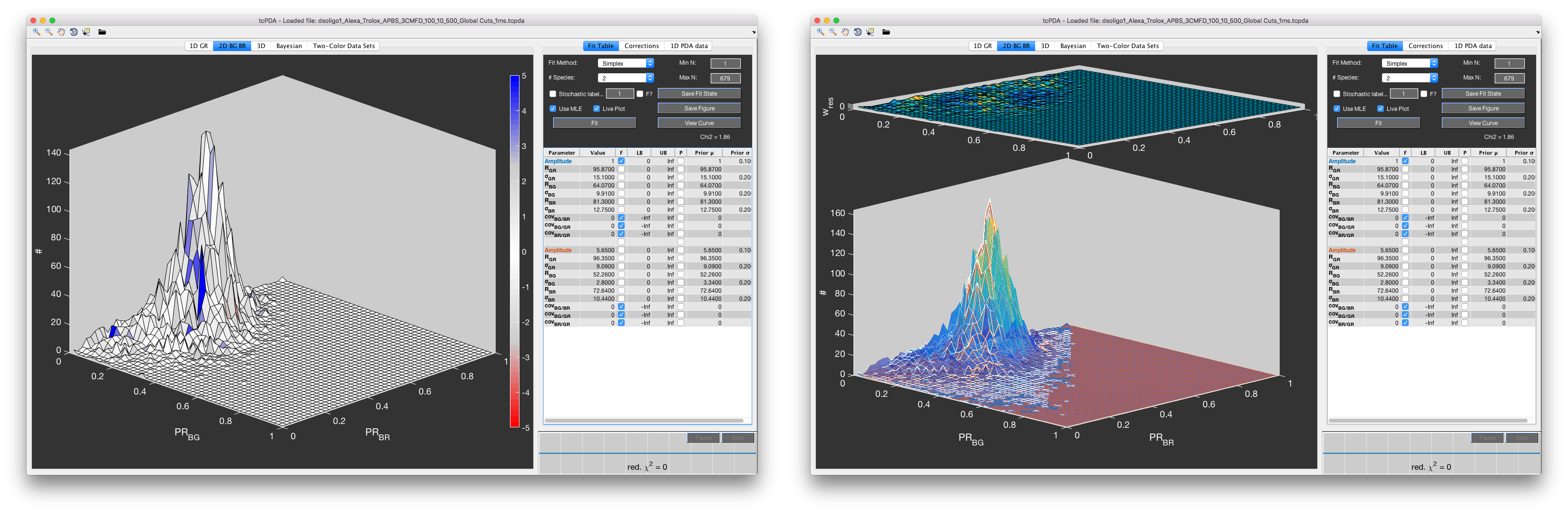
Fitting the two-dimensional histogram of the proximity ratios BG and BR. Left: Colormap-representation of the weighted residuals. Right: Mesh-plot of the fit result.
Similarly to the 1D GR tab, the 2D BG BR tab is used to fit the two-dimensional distribution of proximity ratios BG and BR. This distribution is sensitive to all three center distances and associated distribution widths, including, albeit indirectly, \(R_{GR}\) and \(\sigma_{GR}\). Leaving \(R_{GR}\) and \(\sigma_{GR}\) as free fit parameters, however, will usually lead to values inconsistent with the related distribution of proximity ratio GR, since this information is excluded from this fit. It is thus required to fix \(R_{GR}\) and \(\sigma_{GR}\), which can be easily done by right-clicking the fit parameter table and selecting Fix GR Parameters. The amplitudes as estimated from the one-dimensional fit may be left free or fixed in this step. Covariances should be fixed in this step and only be refined after center distances and distribution widths have been reasonably fit.
As for the 1D GR tab, the fit is always performed using Monte Carlo simulation of the histogram with the Simplex fit algorithm, regardless of the fit options set in the Fit Table tab.
Fitting the full three-dimensional histogram of photon counts
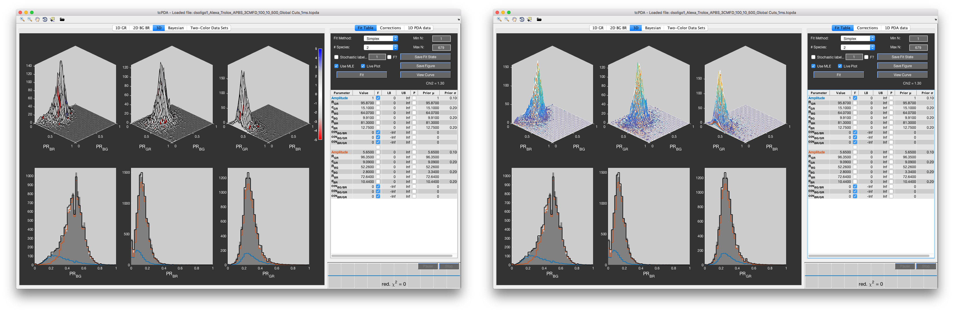
Fitting the full three-dimensional histogram of the proximity ratios GR, BG and BR. Left: Colormap-representation of the weighted residuals. Right: Mesh-plot of the fit result.
The determined parameters should now reasonably describe the data and the refinement of the fit can be performed first using Monte Carlo simulation of histograms. This step is necessary since the maximum likelihood estimator (MLE) will return zero likelihood when the parameter values are too far from their optimum value. Once a region of high likelihood has been reached, one can switch from the Monte Carlo estimation to the MLE. To check if an area of high posterior density has been reached, enable the Use MLE checkbox and confirm that the reported log-likelihood logL is not -Inf.
For the fitting of the full three-dimensional histogram of photon counts, it is advised to iteratively fix and un-fix parameters. Start e.g. by leaving only the center distances as free parameters, after which the distribution width can be fit. Shortcuts for the fixing and un-fixing of groups of parameters are available by right-clicking the fit parameter table. As a final step, un-fix the covariances. Using the Simplex algorithm, covariances will usually not diverge from their initial zero values. Instead, try using the gradient-based or pattern search fit algorithms to fit the covariances. Finally, all parameters should be left free and refined simultaneously. This step can be time consuming, but is essential to ensure that the obtained result is the correct minimum.
Options and settings
Left: Options related to the fit procedure. Right: Display of the photon count distribution found in the Corrections tab.
Fit options
A number of options are available regarding the fit routine and model function.
To switch between using the likelihood expression or \(\chi^2_{red.}\) estimator, use the Use MLE checkbox. If checked, the likelihood expression is evaluated and used as the objective function of the fit routine. If unchecked, the \(\chi^2_{red.}\) estimator is used based on Monte Carlo simulation of the shot-noise limited histograms. In this case, the Monte Carlo Oversampling parameter in the Corrections tab determines the used oversampling factor.
The Fit Method dropdown menu allows to choose between different optimization algorithms. If the 1D GR or 2D BG BR tabs are selected, the Simplex method is always used, regardless of the choice in the Fit Method dropdown menu.
The following fit methods can be chosen:
- Simplex:
- Based on the fminsearch function of MATLAB. To allow to set lower and upper parameter bounds, the fminsearchbnd function from the MATLAB File Exchange is used instead.
- Pattern Search:
- Based on the patternsearch function of the Global Optimization Toolbox of MATLAB. This function is less likely to be trapped in a local minimum than the Simplex option.
- Gradient-based:
- Based on the fmincon function of MATLAB. Uses gradient-based optimization algorithm and is thus generally faster to converge than the Simplex algorithm, but poses a higher risk to end in a local minimum.
- Gradient-based (global):
- Based on the GlobalSearch algorithm of the Global Optimization Toolbox of MATLAB. Similar to the Gradient-based fit algorithm, but performs multiple optimization runs using the fmincon routine using randomized starting points.
The options related to the model function are:
- # Species:
- Specify the number of species of the model function.
- Stochastic labeling:
- Toggle the use of the stochastic labeling correction. This option includes a second population for every species with permuted distances \(R_{BG}\) and \(R_{BR}\). Use this option if not all fluorophores are attached site-specifically. The current implementation assumes that the blue fluorophore is attached site-specifically, but that the two acceptor fluorophores are stochastically distributed over the two possible label positions. Specify the value for the fraction F of the species matching the distance assignment in the fit table using the edit box. The permuted species then has contribution (1-F). To fix the stochastic labeling fraction, toggle the F? checkbox. If unchecked, the stochastic labeling fraction is optimized by the fit routine as a free parameter, taking the specified value as the initial value.
Options that affect the computation time are:
- Min N:
- Exclude time bins with less photons than the specified value. Inspect the photon count distribution shown at the bottom of the Corrections tab to judge the effect of this selection.
- Max N:
- Exclude time bins with more photons than the specified value. Inspect the photon count distribution shown at the bottom of the Corrections tab to judge the effect of this selection.
- Monte Carlo Oversampling:
- Increase this value to reduce statistical noise in the simulated histograms due to the random number generation. The Monte Carlo sampling step will be performed N times, and the final histogram is divided by N.
Display options
- Live Plot:
- If checked, the plots and fit parameter table will update at every fit iteration. If Use MLE is checked, only the fit parameter table is updated since the theoretical histogram is not calculated during the fit process. The Live Plot option will slow down the fit routine due to the time it takes to update the plots.
- Plot type:
- This option is found in the Corrections tab. Specify the way that two-dimensional histograms are plotted. The Mesh option will plot the data as a surface and show the fit function as a mesh. For the 2D BG BR tab. the weighted residuals are plotted above (see here). The Colormap option will plot only the data in the two-dimensional plots. Weighted residuals are shown using a colormap on the data in a range between -5 and 5, color-coded from red over white to blue. See here to see the effect of this option on the 3D tab.
- # Bins for histogram:
- Specify the number of bins per dimension used to histogram the data. Since a higher number of bins will result in less counts per bin overall, one should also increase the Monte Carlo Oversampling* parameter when increasing the number of bins to counteract the increased noise due to the reduced sampling.
Saving the fit state
Saving the current settings and fit parameters using the Save Fit State button will store all information in the .tcpda file. To save different fit states for the same file, right-click the Save Fit State button and select Save Fit State in separate file to store the parameters in a .fitstate file. To load a fit state from an external file, right-click the Save Fit State button and select Load Fit State from separate file. Loaded two-color PDA data sets are also saved upon saving the fit state.
Exporting figures
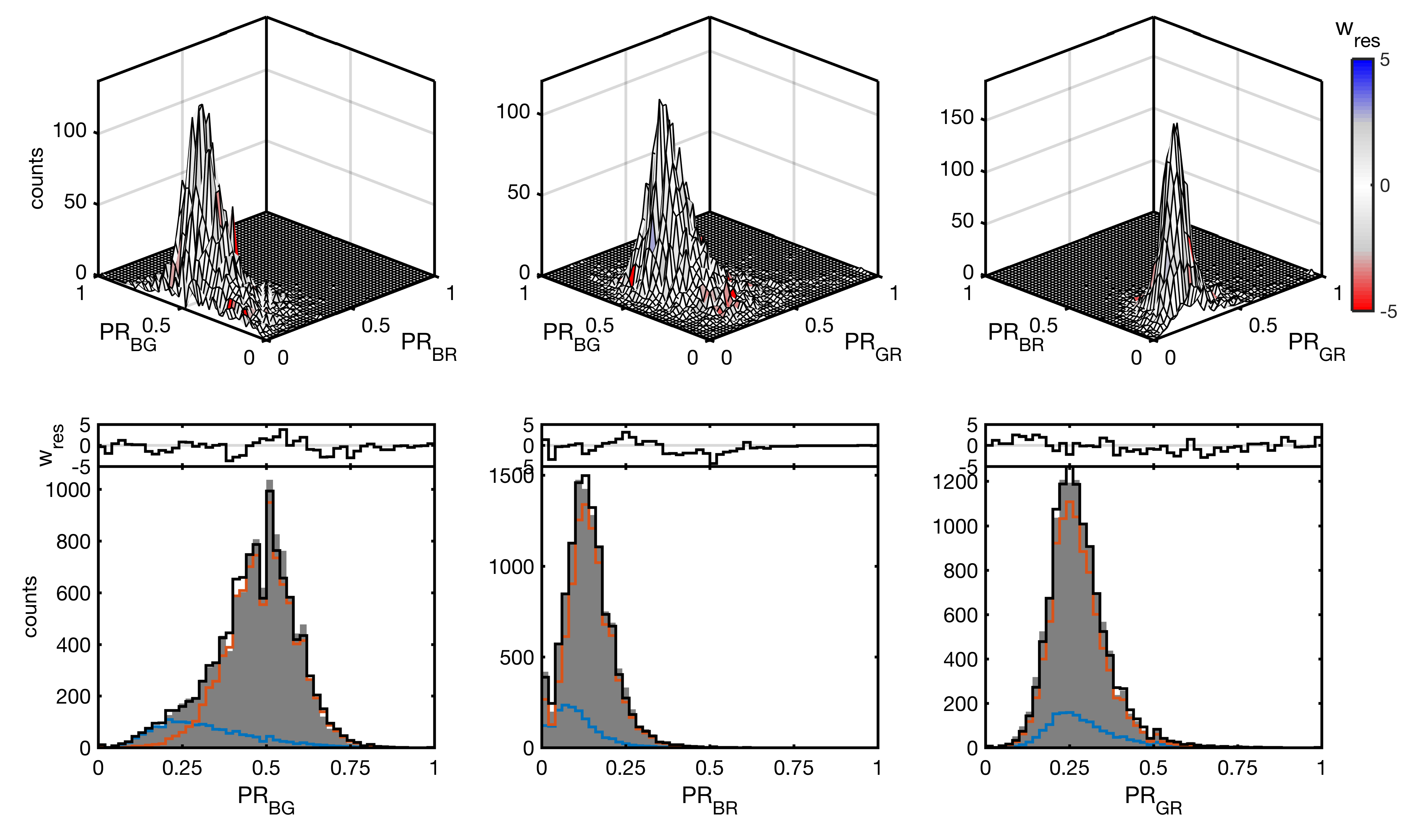
Exported figure of the fit result.
To export the fit result to a figure, click the Save Figure button. This will open a new figure window and plot the currently displayed photon count distribution using the colormap display option. Additionally, a second plot will be generated showing the extracted distance distributions and correlation coefficients between the three distance dimensions.
Note
Before exporting a figure, re-generate the simulated histogram using a high value for the Monte Carlo oversampling parameter to reduce stochastic noise.
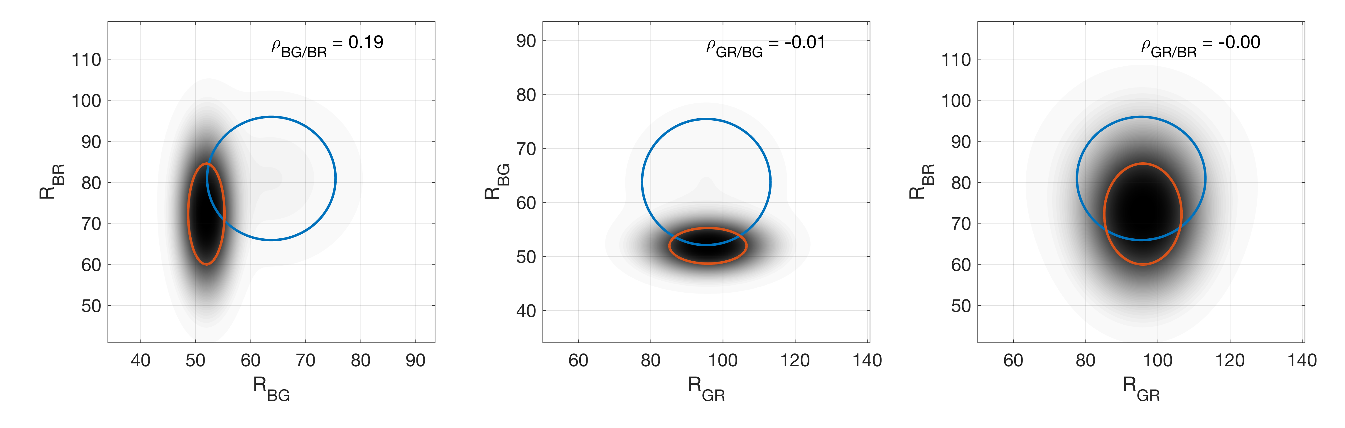
Marginal distributions of the fitted distance distribution. Correlation coeffcients between the distance pairs are given in the top right of the plots. Colored circles indicate \(1\sigma\) levels of the individual species.
Using prior information
In the Bayesian framework, prior information about the parameters can be included into the analysis by the prior distribution:
Here, \(P(\theta|D,I)\) is the posterior probability of the parameter vector \(\theta\) given the data \(D\) and the background information \(I\), which is proportional to the probability of the data given the parameters, \(P(D|\theta)\), multiplied by the prior distribution of the parameters given the background information, \(P(\theta|I)\).
In tcPDA, one can assign normal prior distribution for each parameter separately using the fit parameter table. Checking the P checkbox for a parameter enables the prior for it. Specify the mean (Prior \(\mu\)) and width (Prior \(\sigma\)) for the parameter as estimated from the available information.
Only normally distributed prior are available, and no correlated information about different parameters is accounted for at the moment.
Estimating confidence intervals
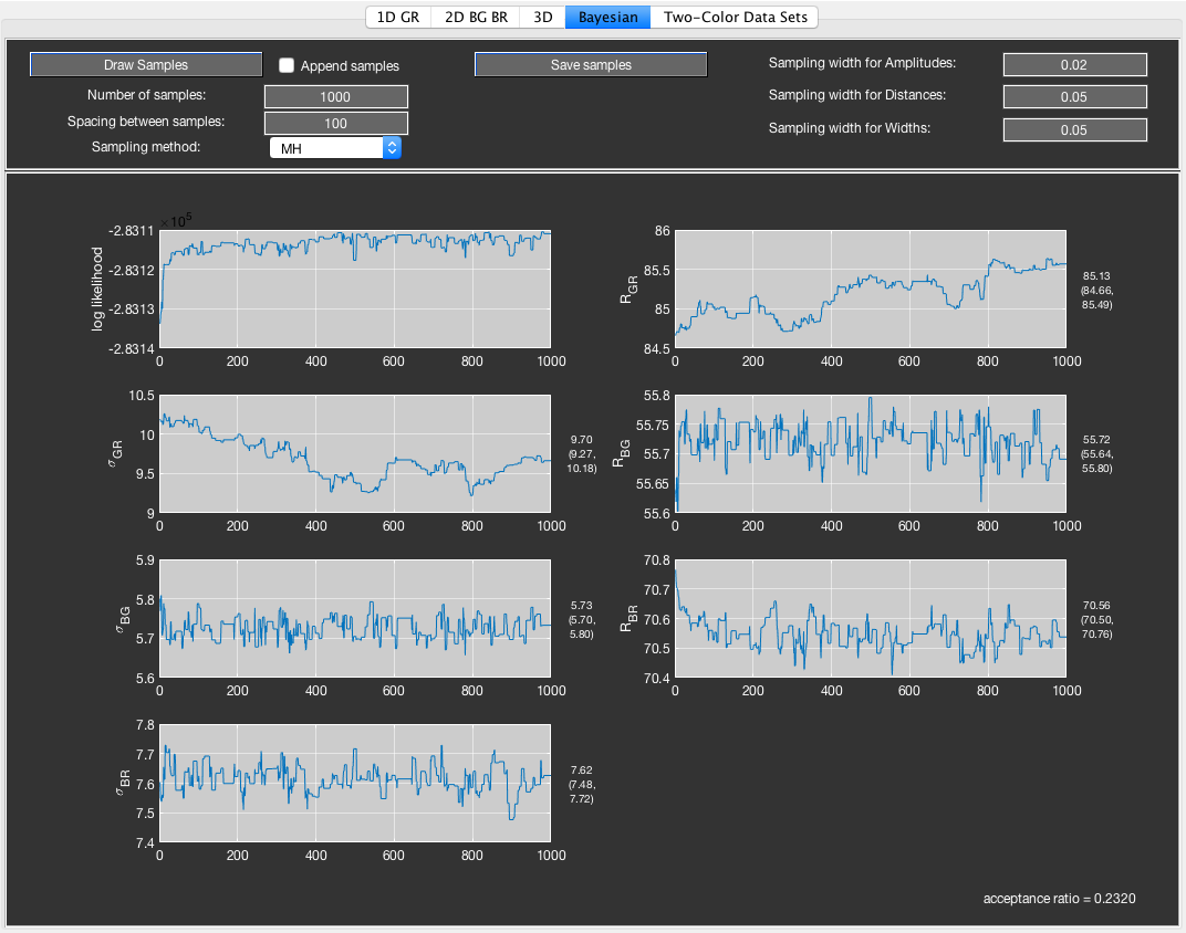
Markov chain Monte Carlo sampling of the posterior probability density.
The Bayesian tab allows to estimate confidence intervals of the fitted parameters using Markov chain Monte Carlo (MCMC) sampling. A random walk is performed over the parameter space. At every step, new parameter values are drawn based on the proposal probability distribution given by a Normal distribution with specified width. The change of the parameter vector is accepted with probability given by the ratio of the likelihoods:
By tuning the width of the proposal distribution, one can adjust the acceptance probability of the random walk, which should fall into the range of 0.2-0.5.
This method to sample the posterior likelihood is called Metropolis-Hasting sampling (called MH in the Sampling method dropdown menu). Additionally, tcPDA implements Metropolis-within-Gibbs sampling (called MWG in the Sampling method dropdown menu). This sampling method performs a Metropolis-Hasting sampling step for all parameters consecutively. The simultaneous re-sampling of all parameters in MH sampling can lead to low acceptance probabilities. By performing the sampling one parameter at a time, the algorithm is less likely to step into regions of low likelihood. MWG is thus to be preferred to MH when many parameters are estimated simultaneously. However, since the likelihood has to be evaluated at every step for every parameter, it is computationally more expensive.
Based on the sampled parameter values, the 95% confidence intervals are determined from the standard deviation \(\sigma\) by \(\mathrm{CI}=1.96\sigma\). To obtain independent samples from the posterior distribution, one can define a spacing between the samples used to determine the confidence intervals.
Click the Draw Samples button in the Bayesian tab to begin drawing the number of samples from the posterior distribution as specified in the Number of samples input field. Drawing samples takes the same parameters and options defined in the Fit table and Corrections tabs as performing a normal fit, with the difference that the MLE is always used. Choose the sampling method between MH and MWG using the Sampling method dropdown menu. When the Append samples checkbox is selected, the newly drawn samples will be added to the previous run of the random walk. Otherwise, previous results will be overwritten. The display will update every 100 steps and show the evolution of the log-likelihood and all free parameters. The acceptance ratio is shown in the bottom right and periodically updated. The sampling width can be set separately for the amplitudes, center distances and distribution width, and can be adjusted to tune the acceptance ratio. Upon completion of the sampling, mean parameter values and 95% confidence intervals will be shown to the right of the parameter plots. Confidence intervals are determined from samples with specified spacing in the Spacing between samples field. This value can be adjusted after the sampling has completed, which will update the displayed confidence intervals. Finally, click the Save samples button to store the result of the MCMC sampling in a text file in the folder of the data.
Global analysis using two-color data sets
tcPDA also implements a global analysis of two- and three-color FRET data sets. This function is useful if the three-color system has previously been studied using two-color FRET experiments with the same labeling positions. Hereby, the fit functions optimizes a global likelihood over all loaded data sets:
The underlying distances are the same between the two- and three-color FRET data sets. However, the correction factors and size of the time bin can be different between the experiments. It is even possible to include two-color FRET information measured using different dyes, assuming that the fluorophores are not influencing the properties of the studied molecule.
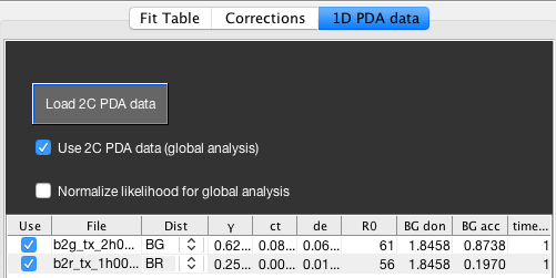
GUI for handling additional two-color PDA data.
Currently, only two-color PDA data exported from the BurstBrowser module is supported (.pda files). The correction factors and time bin are read from the .pda file, but can be modified in the table as well. Every two-color data set needs to be assigned the corresponding distance in the three-color FRET system (GR, BG or BR). Toggle the use of a specific data set by unchecking the Use checkbox in the table. Loaded two-color data sets are stored when the fit state is saved. The two-color FRET data sets are shown in the Two-color Data Sets tab.
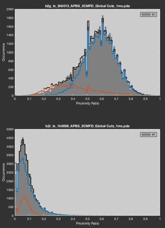
Display of the fit results for additional two-color FRET data sets.
Check the Use 2C PDA data (global analysis) to include the two-color information in the fit. The Normalize likelihood for global analysis checkbox will use the geometric mean of the individual likelihoods to assign equal weight to each data set:
Consider that using many two-color FRET data sets with this option will reduce the overall contribution of the three-color data set.
Note
Note that, while information on the center distances, population sizes and distribution widths is shared between two- and three-color data sets, the correlated information is unique to the three-color data set. Thus, the use of the global analysis is expected to increase the robustness of the extracted correlated information.
Considerations for fit performance
Monte Carlo simulation of histograms
The number of bins for the histograms affects this fitting procedure. The Monte Carlo oversampling parameter, found in the Corrections GUI, will reduce noise and thus improve the convergence of the fitting procedure, however the computation time will scale linearly with this parameter. For initial fitting, a value of 1 may be chosen to quickly find the optimal region. Upon refinement, the value should be increased to 10 or higher.
The simulated histograms are used to represent the fit result also when the MLE procedure is used. To export a plot of the final histograms, showing the result of the analysis, consider using a high oversampling factor of 100 to obtain theoretical histograms that are not affected by noise.
Maximum likelihood estimator
The MLE is unaffected by the number of bins used for this histograms or the Monte Carlo oversampling parameter. However, the performance of the likelihood calculation critically depends on the background count numbers. Try to keep the background signal low to improve performance of the algorithm.
The performances decrease in presence of high background count rates because the total likelihood is given by the sum over all likelihoods given the possible combinations of background and fluorescence photon counts. Since three channels are present in three-color FRET, the number of likelihood evaluations is thus given by the product of the number of background counts to consider per channel, which quickly grows to significant excess calculations.
Consider for example a background count rate of 1 kHz per channel and a time bin size of 1 ms, corresponding to an average background count number of 1. By accounting for the probabilities of 0, 1 and 2 background counts, given by a Poissonian distribution, one accounts for more than 90% of the possible background count occurrences. Still, the trinomial distribution would have to be evaluated \(3*3*3=27\)-times more often (and the binomial distribution 9-times more often) compared to when no background signal were present.
CUDA support
The likelihood estimator is available for use with NVIDIA GPUs. By default, the program will look for available CUDA-compatible graphics cards and default to the CPU if none are found.
For use in MATLAB, the CUDA code is compiled into a MATLAB MEX file and available for the Windows and Linux operating systems. If the supplied MEX file does not work, follow the instructions in the help file found with the source code to re-compile the MEX file on your computer.
| [Barth2018] | Barth, A., Voith von Voithenberg, L., & Lamb, D. C. (2019). Quantitative Single-Molecule Three-Color Förster Resonance Energy Transfer by Photon Distribution Analysis. J Phys Chem B, 123(32), 6901-6916. https://doi.org/10.1021/acs.jpcb.9b02967 |