Microtime Image Analysis (MIA)

Contents

• Microtime Image Analysis (MIA)
  • Data loading and handling
    • Options tab
  • Main Image Tab
    • Channels
    • Image
    • ROI
    • Correction
    • Correlate tab
    • N&B tab
    • FRET tab
    • Co-localization tab
  • Additional information tab
  • (R)ICS tab
  • TICS tab
  • STICS/iMSD tab
  • Number and Brightness tab
    • Converting analog to photon counting data
  • Spectral RICS
  • RICS Performance Evaluation
  • References

The MIA window can be opened from the PAM main window by clicking on Advanced Analysis -> MIA or from the command window by typing in Mia.

MIA is used for a variety of different image analysis methods, mainly via image correlation techniques.

Sample data for different types of analyses can be found here: https://gitlab.com/PAM-PIE/PAM-sampledata

An introduction and description of the various techniques can be found in:

Image Correlation Spectroscopy (ICS): [Petersen1993]

Image Cross-Correlation Spectroscopy (ICCS): [Wiseman2000]

Raster Image Correlation Spectroscopy (RICS): [Digman2005] and [Digman2009a]

Spatio-Temporal Image Correlation Spectroscopy (STICS): [Toplak2012]

Image Mean-Square Displacement (iMSD): [DiRienzo2013]

Number & Brigthness (N&B): [Digman2008] and [Digman2009b]

Combination of Pulsed Interleaved Excitation and Fluctuation Imaging (PIE-FI): [Hendrix2013] and [Hendrix2015]

Arbitrary Regions for Image Correlation Spectroscopy (ARICS): [Hendrix2016]

Spectrally resolved RICS: [Schrimpf2018]

Performance evaluation for RICS: [Longfils2019]

MIA main gui

Data loading and handling

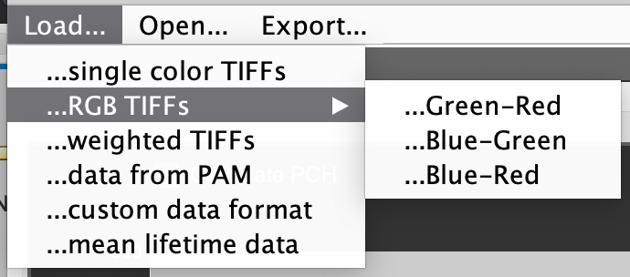
The loading menu

MIA supports different kinds of input data.

Menu Load…

single color TIFFs: A popup window appears to select grayscale TIFF files to be loaded (multiple files will be concatenated). The file selection window will be opened a second time to select the files for the second channel. Press cancel if only one color is needed.

RGB TIFFs: A popup window appears to select RGB TIFF files to be loaded (multiple files will be concatenated). Depending on which menu item is chosen, the RG, RB or GR channels from the TIFF file are loaded.

data from PAM: Accessing the files currently loaded in PAM to generate an image series, using the PIE channels defined in the Channels tab.

weighted TIFFs: For loading lifetime-resolved [Hendrix2013] or spectrally-resolved [Schrimpf2018] data. This works the same as standard TIFF data, but extracts re-scaling parameters from the data to account for the non-integer values saved with an integer file format. RLICS and RSICS TIFFs contain the unfiltered data in the first half and the filtered frames in the second half. This option loads only the filtered frames (the raw data can be loaded with the normal single color TIFFs option).

custom data format: This case depends on the particular format selected. To change the custom read-in to the desired format, go to the Options tab. and change the Custom Filetype dropdown menu.

If you have analog data, you can click the y axis label in the count rate plot to display the axis in counts instead of absolute photon counts (kHz). Alternatively, you can convert analog to photon counting images or select the analog checkbox on on the Options tab.

All data is stored in the global variable MIAData and can be easily accessed from the MATLAB command line.

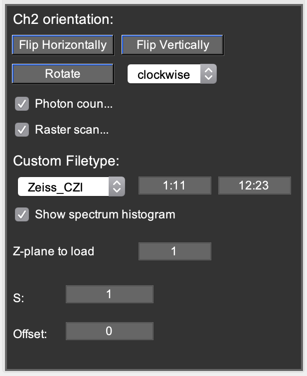
Options tab

The options tab

Miscellaneous options related to data loading and conversion prior to any analysis are grouped here.

Ch2 orientation: This option can be used to flip or rotate an image in case e.g. cameras were rotated with respect to each other.

Photon counting: Checking it will display all count rate values in kHz. Unchecking it will display counts in arbitrary units.

Raster scanning: Checking it will display the pixel dwell time and line time on the Image tab and converts pixel counts to kHz when calculating count rates. Unchecking it does not rescale pixel counts when calculating count rates.

Custom filetype: Here, the user can define specialized read-in routines. For Zeiss .czi files, use the Zeiss-CZI option. In the leftmost (rightmost) editbox, define the spectral channels summed into the top (resp. bottom) image channel of Mia. 1:11 means summing up spectral channels 1 to 11. The Show spectrum histogram option can be used to verify in which spectral windows the sample fluoresces.

Z-plane to load (only visible when the Zeiss-CZI option is selected): allows extracting specific planes from a multi-plane .czi file. You can also define a range of z-planes by writing e.g. 1:5 or 1,2,5. To allow correct blockwise RICS analysis of a z-stacks, Mia will automatically adjust the frame range (ROI tab) and Window/Offset on the Correlate tab.

S & Offset: Here, the parameters from [Dalal2008] can be entered to convert analog to photon counting images.

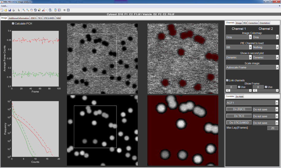
Main Image Tab

The central controls and settings of MIA are found in the Image tab. The two leftmost plots show the mean frame intensity and a photon counting histogram. The green lines correspond to the first and the red to the second channel. The dotted lines represent the data for the full stack, while the solid line represents the selected pixels in the region of interest (ROI) after correction. A mouse click on the y-label toggles different displaying options.

The four images in the center show the full frame (left) and the selected and corrected ROI (right) for the first (upper images) and second (lower images) channels. On the leftmost images, the ROI is drawn via a solid square or rectangle.

The image tab

Hint

All images in MIA can be exported as 8bit RGBs with the same contrast as displayed.

• Leftmost images:

  • “left-click”: center ROI
  • “ctrl”+”left-drag” or “right-drag”: draw normal ROI
  • “shift”+”left-click” or “middle-click”: export image.
  • if the ‘Left Image Context Menu’ checkbox on the ROI tab is checked, an arbitrary ROI can be drawn via “right-click” on the image

• Rightmost images:

  • “right-click”: draw AROI popupmenu
  • “shift”+”left-click” or “middle-click”: export image
  • “right-click” on the rightmost images gives a context menu for manually drawing an arbitrary ROI using “left-drag”

• Dual color images or videos:

  • Can be generated using the “Export” Menu

All settings for displaying, correcting and analyzing the images can be found in the various tabs at the right of the window, and will be individually discussed in the next sections.

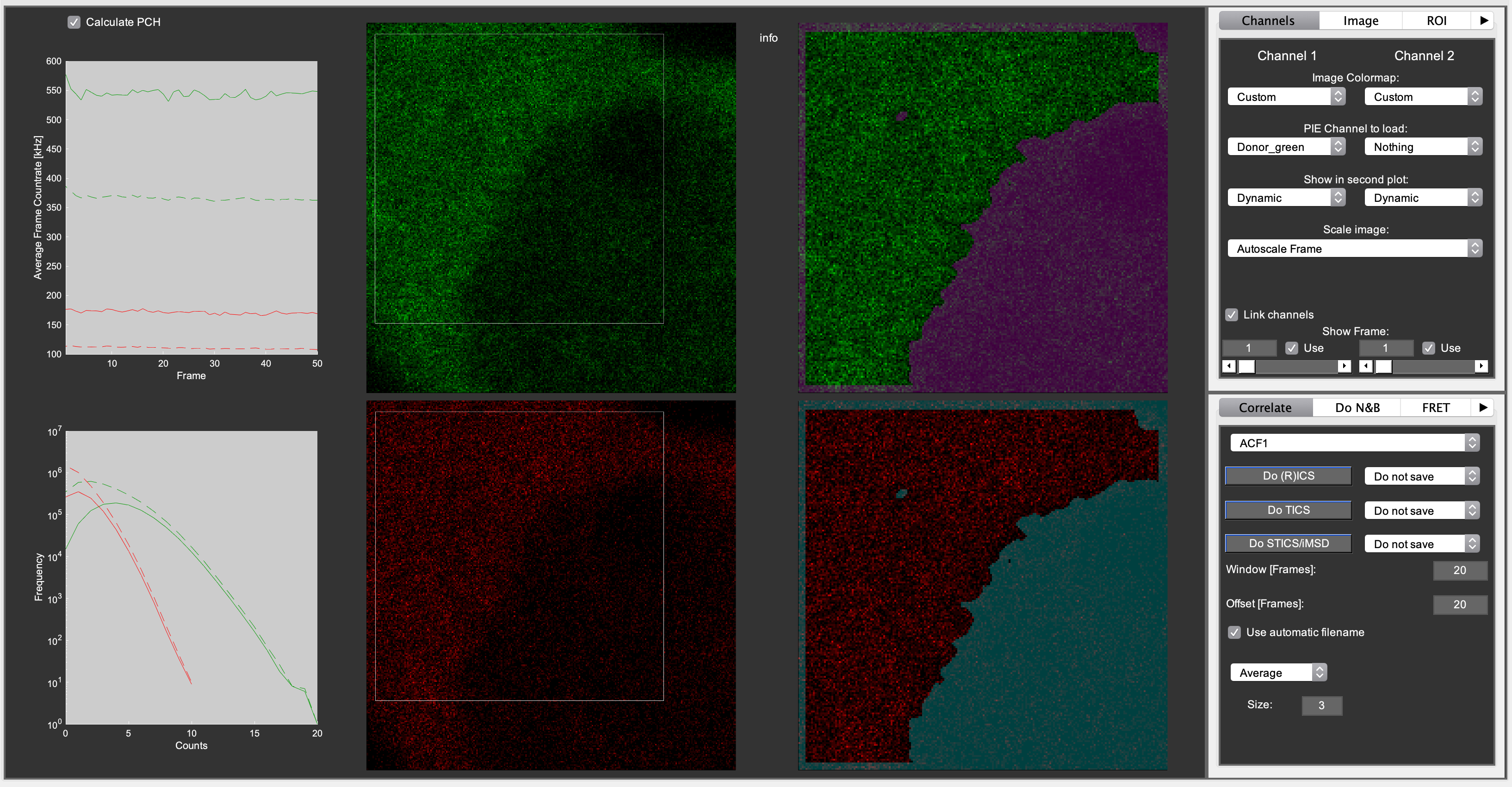
Channels

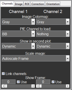
The channels tab

This tab contains mainly setting for displaying the images and switching between frames. From top to bottom these are:

Image Colormap:

This changes the colormap for the channels between different options to standard MATLAB colormaps (Gray, Jet, Hot and HSV). The HiLo colormap is the same as the Gray colormap with the exception that all pixels below and above the manual scaling are displayed in blue and red, respectively. The Custom colormap uses a single color (standard green and red) for displaying. The color can be changed with the middle mouse button.

PIE Channel to load:

This function selects the PIE channel that will be used when data is loaded from the PAM main window. For the second channel Nothing can be selected for one channel analysis.

Show in second plot:

This option switches between different options to display in the right images. Original and Dynamic show the ROI before and after the corrections are applied, respectively. Static show the corrections that were applies, i.e. the difference between Original and Dynamic.

Scale Image:

This switches between different scaling options. Autoscale Frame scales the image to the min/max of the displayed image, while Autoscale Total scales to the min/max of the full stack. Manual Scale allows the users to set their own fixed scaling limits.

Link channels:

This checkbox (un)links the two channels, so that the frames can be changed individually or together.

Show Frame:

These edit boxes and sliders are used to switch between different frames of the stack. When frame “0” is selected, the program displays the mean of Frame range displayed on the ROI tab. With the Use checkbox the user can unselect individual frames for some further analysis.

Image

This tab contains the most important information about the image stacks, like frame, line and pixel time and the pixel size. These values are used for certain calculations and data processing. If the metadata contain information on any of these parameters, these values will be updated automatically.

Scale bar: Enter any value to display the scale bar on the images. If the entered value is too large, Mia will automatically make the scale bar fit within both the left and right images. Enter 0 or no value to hide the scale bar. Scale bars are included in the exported images.

ROI

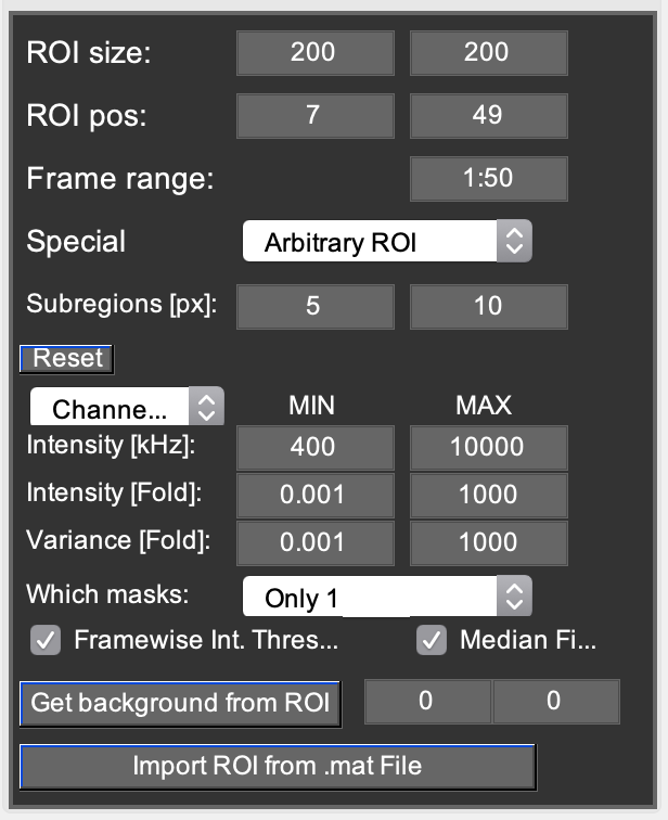
The ROI tab

This tab contains options for selecting ROIs and discarding pixels vie arbitrary region ICS. From Top to bottom:

ROI size and position:

These edit boxes define the size and position of the selected ROI for both channels. Alternatively, the user can click on the left images to position the ROI. Right-dragging the leftmost images also allows drawing the ROI box. Left clicking shifts the center of the current ROI without changing the size.

Frame range:

This allows the user to define the frames used for most further data processing. This uses standard MATLAB notation for array slicing. When frame 0 is selected on the %%Channels%% tab, Mia displays the average image calculated from this frame range.

Special popupmenu:

This popupmenu switches between (1) using all frames within the frame range, (2) using the frames within the frame range that have a checked Use checkbox on the Channels tab, or (3) using arbitrary region ICS for further data processing. Arbitrary region ICS ([Hendrix2016]) allows discarding individual pixels from the correlations to remove the influence of unwanted objects and artifacts from the analysis. There are different ways of unselecting pixels, which can be combined.

Subregions [px]:

Further options below employ the mean property of pixels in one or two small ROIs within the image. The size of those small ROIs is defined by these two edit boxes. The left size always has to be smaller than the right size.

Reset pushbutton:

This button resets all AROI selection values to their defaults.

Channel popupmenu:

Allows switching between the AROI values for channel 1 or channel 2, as these will be different.

Intensity [kHz]:

Pixels are discarded if their mean intensity throughout the whole stack falls outside the range defined by MIN and MAX. A value equal to zero for MIN and MAX turns it off. This is especially useful for discarding e.g. the cell exterior.

Intensity [fold] or Variance [fold]:

The intensity or intensity variance inside the small Subregions ROI is compared with the large Subregions ROI. If the ratio between those values is below or above the range defined by the values in the edit boxes, the pixel is discarded. For pixels at the edges the ROI cannot be created. These pixels are therefore automatically discarded. Note: These options are performed on a frame to frame basis, so pixels are not automatically removed from the whole stack. Pixels that use discarded pixels for a moving average subtraction/addition are also discarded.

Which masks popupmenu:

Independent: Masks are generated per channel. Note: resulting analysis may be performed for different pixels in channel 1 and 2.

Only 1 (2): The mask for channel 1 (resp. 2) is automatically applied to channel 2 (resp. 1), the other channel’s mask is ignored. 1&2: Only pixels included into the mask of both channels are kept. All other pixels are excluded from the mask.

Framewise Int. Threshold:

Pixels are discarded on a framewise basis if their mean intensity in the small Subregion falls outisde the range defined by MIN and MAX. Note: The intensity in the small subregion is rescaled (/(mean int.frame)*(mean int.frame1) to account for intensity fluctuations such as drift or photobleaching.

Median Filter:

Smoothens the arbitrary ROI by applying a 3x3 median filter.

For all arbitrary region ROIs, unselected pixels are highlighted in the right images, based on the selected colormap.

An arbitrary ROI can also be manually drawn onto any image. Once Arbitrary ROI has been selected in the Special popupmenu, Right-clicking the corrected image will display a menu. When Select manual ROI is chose, holding down and dragging with the left mouse button will draw an AROI on the image. The selection applies throughout the stack. Drawing an AROI on the left image is also possible by checking the ‘Left Image Context Menu’ checkbox.

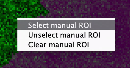
The AROI drawing menu

Get background from ROI pushbutton:

For some applications (e.g. RICS or N&B) it might be useful to subtract the background from the corrected image prior to further analysis. Pushing this button displays the average count rate (in photons per pixel dwell time) in the currently selected ROI. Alternatively, if you know the background count rate from a control experiment, you can also write the value directly in the edit box. The left edit box is channel 1, the right one is channel 2. The values displayed in the edit boxes are subtracted from the images after any correction (see Correction tab) has been carried out.

Import ROI from .mat file pushbutton:

Allows importing a mask from a pre-defined .mat file. This file can be generated manually, or in the N&B tab. It has to have the following content: % ROI = [sizeX sizeY posX PosY] % Mask = ROI-sized single frame mask

Correction

This tab has options to apply corrections to the data, e.g. to get rid of an immobile fraction for (R)ICS. It includes various options for subtracting from and adding to the image, including a moving average (both pixels and frames), and pixel, frame and total mean. For the calculation of these values the discarded pixels from the arbitrary region selection are not used.

For RICS analysis, typically a pixel-based 3-frame (from frame-1 to frame+1) moving average subtraction (Pixels: 1 and Frames: 3) and a total mean addition are typically used [Hendrix2015]. Correlation amplitude bias due to this correction is undone [Hendrix2016].

For N&B analysis, typically a box-based moving average subtraction (e.g. Pixels: 3 and Frames: 3) and a pixel mean addition are typically used [Hendrix2015].

For TICS analysis, typically a frame mean subtraction and a total mean addition are typically used to correct for slow intensity drift [Hendrix2015].

Drift correction: Correction for linear lateral drift of the sample. When checked, Mia cross-correlates every frame with the first one and using the (x,y) position of each of the crosscorrelation functions, it laterally translates each frame relative to the first one. A graph of the x,y offset of the crosscorrelations is also plotted.

Correlate tab

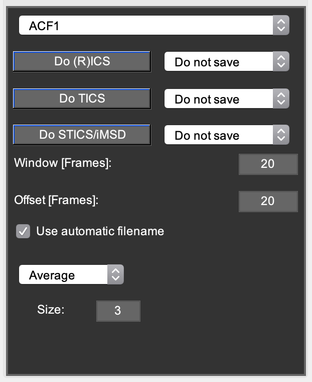
The Correlate tab

At the bottom right of the main window is a tab that contains all settings and buttons for applying the various ICS methods like (R)ICS, TICS, STICS and iMSD.

In the first popupmenu, the user can choose to calculate only a single autocorrelation function for the selected channel, or both auto- and crosscorrelation functions. Additionally, the user can choose for each method whether and how to save the calculated data.

Two extra edit boxes are present: Window and Offset.

(R)ICS using the ‘save blockwise analysis as .miacor’ option.

• Window is the window size (in frames) in which correlation data need to be averaged
• Offset is the offset (in frames) of the next window with respect to the previous.

• For analyzing adjacent windows, Offset = Window. For example:

  W=50, O=50 analyses the data from frame 1-50, 51-100,… W=50, O=10 analyses the data from frame 1-50, 11-60,…

• Blockwise analysis can also applied to individual z-slices from .czi files containing z-stacks. For example:

  Suppose there’s 5 z-slices and 50 frames per slice, and a moving average correction of 3 frames is used. On the ROI tab in frame range, take 2:250 instead of 1:250 On the Correlate tab: W=48, O=50 analyses the data from frame 2-49, 52-99,…, this way effectively omitting the wrongly corrected frames 50 and 51 in between different slices. Suppose there’s 5 z-slices and 50 frames per slice, and a moving average correction of 4 frames is used. On the ROI tab in frame range, take 2:250 instead of 1:250 On the Correlate tab: W=47, O=50 analyses the data from frame 2-48, 52-99,…, this way effectively omitting the wrongly corrected frames 49-51 in between different z-slices.

STICS/iMSD

• Window is the maximum number of lags (in frames) that have to be calculated.

The popupmenu: ‘None’, ‘Average’, ‘Disk’, ‘Gaussian’.

Spatially averages TICS correlations to improve statistics. The size (in pixels) can be entered in the respective checkbox

N&B tab

The N&B tab

The popupmenu: ‘None’, ‘Average’, ‘Disk’, ‘Gaussian’.

Applies an averaging filter to the intensity and variance images used for N&B analysis. The size (in pixels) can be entered in the respective checkbox.

Median filter.

Applies a median filter to the resulting N and epsilon images on the N&B tab

Detector dead time [Hendrix2013]

Enter a value here if a detection system (e.g. TCSPC or APD detectors) with non-negligible dead time is used for aqcuiring the data.

FRET tab

Used to calculated acceptor/donor FRET. Temporary version.

Co-localization tab

Used to calculate the Pearson’s colocalization. Temporary version.

Additional information tab

This tab contains a couple of plots that show general information about the loaded files in greater detail. The left hand side shows the data as a frame average, while the right side shows the time average.

(R)ICS tab

The third window is reserved for displaying the image correlation data and a quick first evaluation of the data quality. Proper analysis is done using the MIAFit sub-program by selecting to save the data as a MATLAB file with a .miacor ending. It is also possible to save the data as TIFFs to load and plot them with standard image analysis programs like ImageJ.

The autocorrelations are plotted in the right and left plots, while the crosscorrelation is shown in the center plots. Hereby, the first row displays the correlations as and image plot. In the second row, it is plotted as a surface plot. The last row displays data related to the fit, either the fit or the residuals as a surface plot. The third option plots the data as a surface and the residuals in blue and red. The last option shows the on-axis data and fit.

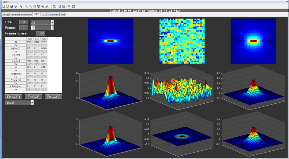
The (R)ICS tab

The setting in the top left define the size of the correlation to be used, the colormap for plotting and which frame to display. When frame “0” is selected, the program displays the average of the frames defined in the Frames to use edit box. Use standard MATLAB notation.

TICS tab

The TICS window is reserved for temporal correlation data and for a quick first evaluation of the data quality. Proper analysis is done using the FCSFit sub-program by selecting to save the data as a matlab file with a .mcor ending. To limit the contribution of undersampling, the correlation is only calculated up to one tenth of the maximum movie length.

The plot at the top of the window shows the pixel averaged auto- (green and red) and crosscorrelation (yellow). The table on the left can be used to perform a very simple 3D diffusion FCS fit.

The three images at the bottom show different calculated correlation parameters for the individual pixels for the two auto- (left and right) and the crosscorrelation (center). The user can select regions of the image by right clicking on them and export the averaged correlation for only the selected region.

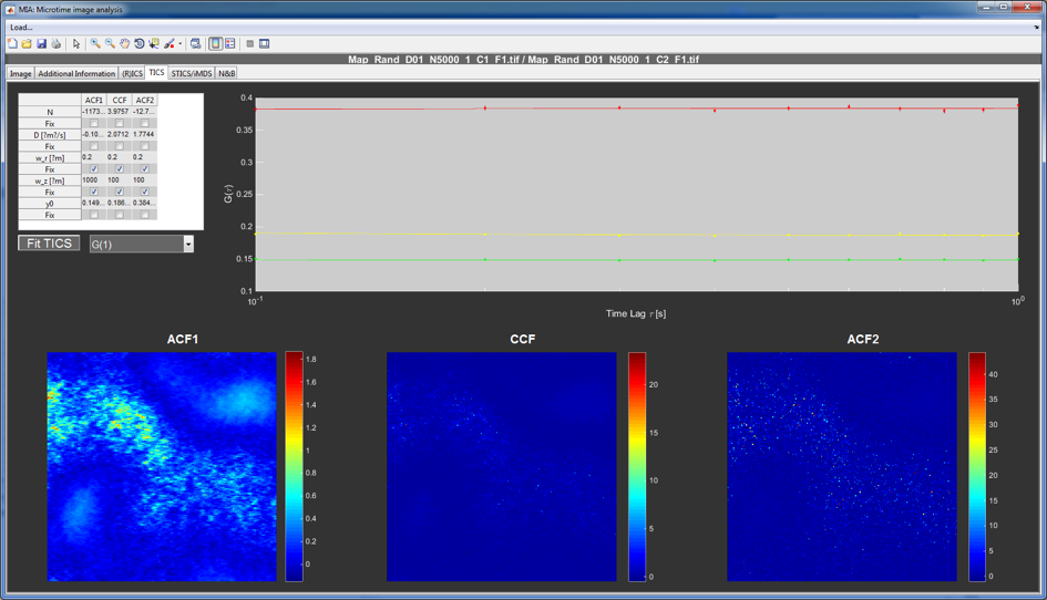
The TICS tab

In the latest version of the TICS tab, different thresholding options are included:

G(1)-G(end): threshold on the basis of the amplitude of the decaying part of the TICS correlation

Brightness: threshold on the basis of Counts*(G1-Gend)

Counts: threshold on the basis of the average pixel intensity. Similar to arbitrary ROI thresholding.

Half-Life: threshold on the basis of the half-amplitude correlation time. This can be used to remove quasi-immobile pixels and other diffusive outliers from the average correlation function

**Samples: threshold on the basis of the number of times each lag of the correlation function for a particular pixel is sampled. This is important when an arbitrary ROI is used for generating the TICS data.

Correlation function popupmenu: The thresholds can be displayed and edited in a correlation-function specific manner.

Image to display popupmenu: By default, the G(1)-G(end) images are displayed, but the different above images can be displayed via the popupmenu.

Median filter: median filters the resulting images (Radius defined on the Correlate tab)

Normalize: normalizes the display of the 1D average TICS correlation graphs between 1 and 0, for better displaying.

Reset: resets the thresholds.

STICS/iMSD tab

MIA can not only perform spatial or temporal correlation but also spatiotemporal correlation. The full STICS data can be properly analyzed with MIAFit when saved as a MATLAB file with the .stcor extension. In the STICS/iMSD tab the user can look at the data as a function of lag time in the three images at the bottom (left and right for the auto- and the central for the crosscorrelation).

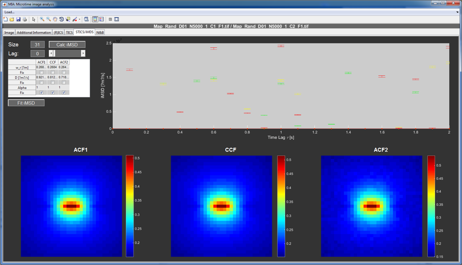
The STICS tab

A simplified way of analyzing spatio-temporal correlation data is called iMSD. Here, the square of the width of the Gaussian used to fit the correlation is plotted vs. the time lag. This way of plotting the data contains in principle the same information as mean-square displacement plots acquired by tracking. The iMSD data can be calculated, plotted and fit with the controls at the top of the window. For a more detailed analysis, the user can select to save the iMSD data during correlation as a MATLAB file with the .mcor extension. Since iMSD gives 1D temporal data, it can be analyzed with an appropriate fit in FCSFit.

Number and Brightness tab

N&B analysis is still under development, so use with caution!

The absolute number and brightness are calculated in Mia from absolute photon counting images using Eqs. 8 and 9 from [Digman2008], with the difference that a one-photon PSF shape correction factor = sqrt(8) is included (Eqs. 16-17 in [Hendrix2015]) to be consistent with RICS analysis.

For analog or pseudo photon counting (e.g. Olympus Fluoview FV1000) data, instead of using Eqs. 8 and 9 from [Dalal2008], in Mia images are converted to absolute photon counting after which Eqs. 8 and 9 from [Digman2008] can still be used.

Data correction:

The N&B program uses the formulas for absolute photon counting A procedure for correcting data prior to calculating N&B can be found in [Hendrix2015]. In brief, for N&B, all slow fluctuations that are not caused by diffusing molecules need to be removed, but, in contrast to RICS, spatial image inhomogeneities due to e.g. concentration differences do not need to be removed. Ideally, subtracting a pixel’s moving average followed by adding the pixel’s average throughout the video would work. In our experience, however, we find it better to subtract the moving average of the ‘local spatial average of a pixel’, followed by adding the pixel’s average throughout the video. Therefore, on the Correction tab in Mia, select

• subtract moving average: pixels = 3, frames = 3
• add pixel mean

Notes:

• Since N&B works on a pixel-by-pixel level, do not select an arbitrary region ROI.
• Any image background correction that you might do will ensure the N&B data is background corrected too.

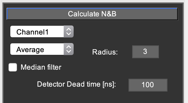
N&B calculation:

On the do N&B tab in Mia, the following options are visible:

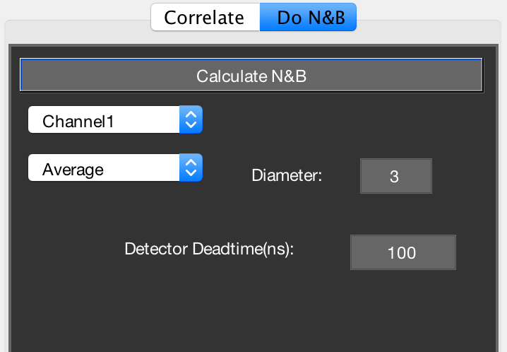
The N&B calculation tab

• Channel 1 popupmenu: select which data channel you want to use for normal N&B [Digman2008], or whether you want to do cross-NB [Digman2009b].
• Average popupmenu: For N&B, the program will calculate the mean and variance image. This option allows you to additionally spatially average (‘smooth’) these images prior to calculating the N&B images.
• Radius: select the smoothing filter radius in pixels.
• Median filter checkbox: applies a [radius x radius] median filter to the N&B images.
• Detector deadtime (ns): as described in [Hendrix2013], detector/TCSPC dead time will cause artifacts in N&B due to the fact that the highest pixel counts are systematically missing some counts, skewing the PCH and thus the N&B data. If you don’t use TCSPC, a value of 0 will probably be ok. If you use TCSPC, look up the device’s dead time. APDs also have a dead time, so take whichever dead time is highest (TCSPC or APD). Hybrid and normal PMTs have very low dead time (~1 ns). If you’re unsure about dead time artifacts, compare the N&B brightness of different concentrations of the same sample (e.g. 10, 50, 250, 1000 kHz). If the brightness artificially goes down, try correcting the dead time to see if the effect disappears.

N&B data display:

On the N&B tab, the calculated N&B data can be displayed and manipulated:

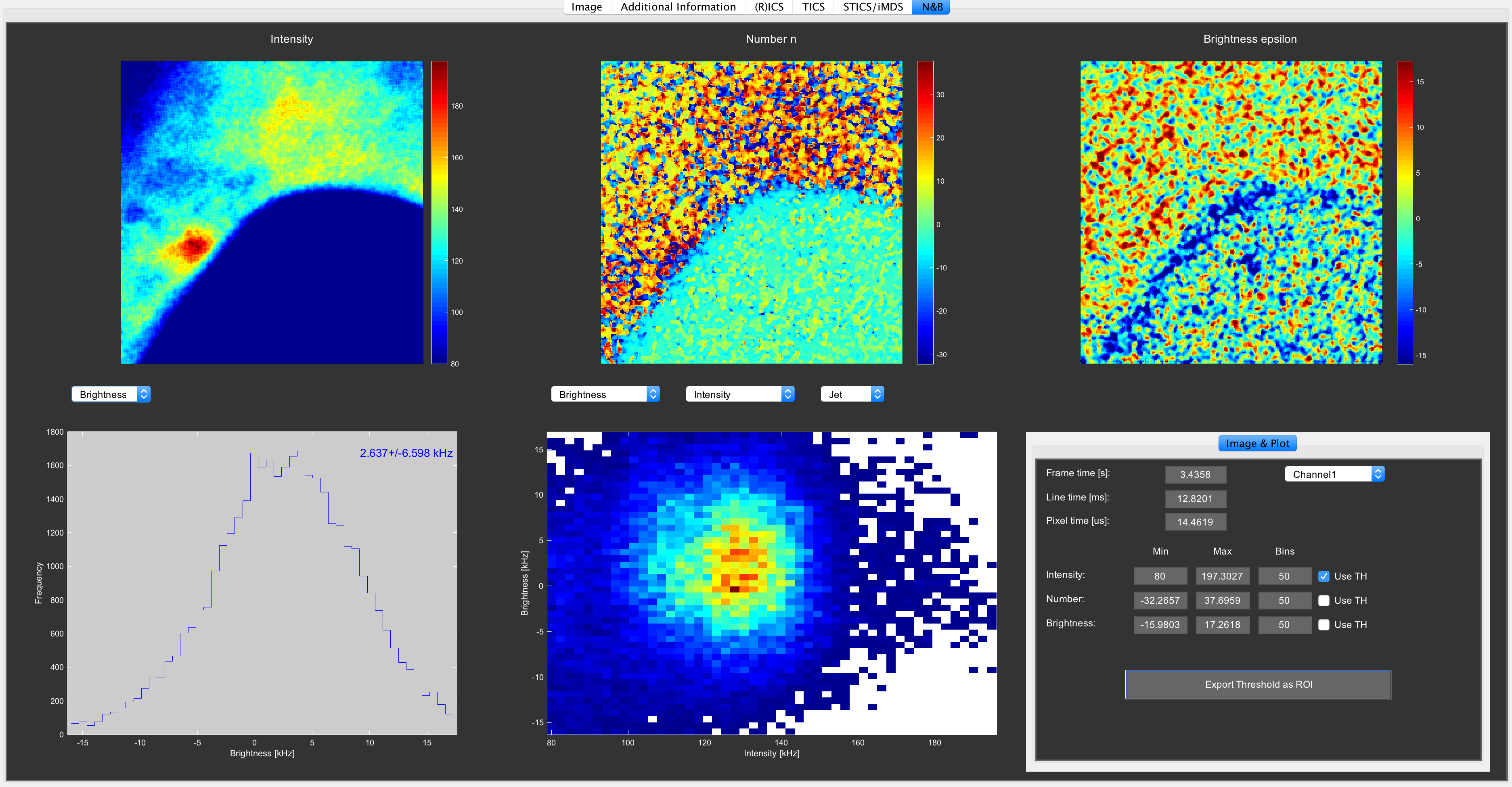
The N&B tab in Mia

• Intensity, number and brightness images display the corresponding parameters in each of the images.
• Intensity, number, brightness and PCH histogram displays the corresponding informations.
• The 2D histogram allows plotting different parameters against each other.
• You can set the thresholds bottom right on the user interface to make the display of the images and histogram look better.
• Clicking the 2D histogram changes the background from white to black
• You can Export the applied thresholds as a mask that can be opened again on the ROI tab in Mia.
• Note: for the correct conversion of pixel counts to kHz, the correct pixel dwell time is needed!

General notes on N&B:

• For a dataset of 100 frames, try to have brightnesses at least >5 kHz, otherwise the data is too noisy for decent N&B.
• Increasing the moving average or filter averaging radi will improve data quality.

Converting analog to photon counting data

For determining absolute brightnesses (kHz) with e.g. RICS and N&B using imaging data recorded in analog mode, and for determining absolute number concentrations with N&B using analog data, the images need to be converted: (Image-offset)/S, with the parameters defined in [Dalal2008]. Here is a brief protocol on how to record the parameters.

• Put a drop of MQ on a coverslip, or MQ in the wells you use for measuring your cells.
• You measure 20 frames with your normal RICS settings 256x256, pixel dwell time 8-20 µs, pixel size ~50nm, BUT instead of using your laser (“unclick” to use the laser), you are creative with light that has different intensity.
• Use roomlight / no light / cellphone light / a bike lamp / … shining in various directions towards your sample. Try to obtain a nice spread in lamp intensity.
• For focussing, (if needed, put something in the well next to it) turn on the laser, 10x higher than usual, put the LUT to see dim signals, and you should find the position where the laser is reflecting the glass, go ~10 µm upwards.
• For analysis, open the file in Mia and simply copy paste the following code to the Matlab command:

global MIAData

disp(['there are ' num2str(size(find(MIAData.Data{1}>255),1)/numel(MIAData.Data{1})*100) ' % saturated pixels']);

int = mean(mean(mean(double(MIAData.Data{1}),3)))

var = mean(mean(var(double(MIAData.Data{1}),0,3)))

• make a variance vs. intensity plot

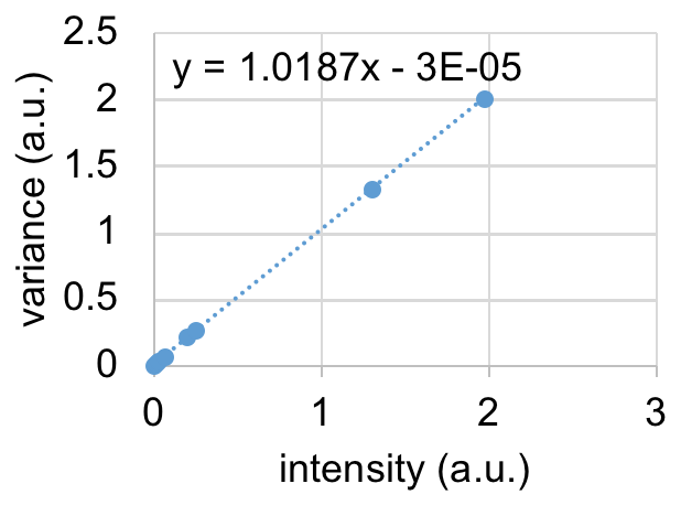
Variance vs. Intensity plot

• Fit a straight line to the data. Slope = S, intercept = offset. Enter those values into Mia. As the data is immediately converted, all downstream calculations are now done on photon counting data.
• Importantly, RICS and N&B analysis should now provide exactly the same number and brightness.

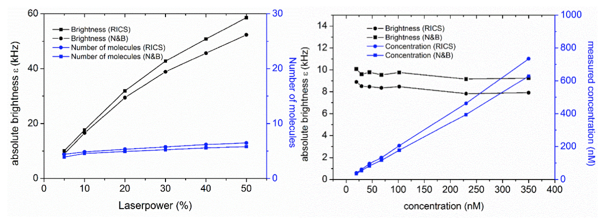
Comparison of RICS and N&B using analog => photon counting converted data (Olympus Fluoview FV1000)

Spectral RICS

From the menu Open… Spectral a user interface can be called that allows generating spectral filters and applying these to RICS data. Alternatively, the Spectral UI can be opened from the command window by typing “Spectral”.

Data can be loaded one by one via Load -> data directly (highlight #1).

For spectral filtering of data, single-species reference data can be loaded via Load -> species data (highlight #1). When selected (highlight #2), the relative frequency of photons detected in the different channels can be observed in the graph.

With the mixed data and pure-species data loaded, by pressing the Create filters pushbutton when both reference species are still selected (highlight #3), filter patterns are created.

In order to process the image series with the spectral filter, go to the Filters tab (highlight #4).

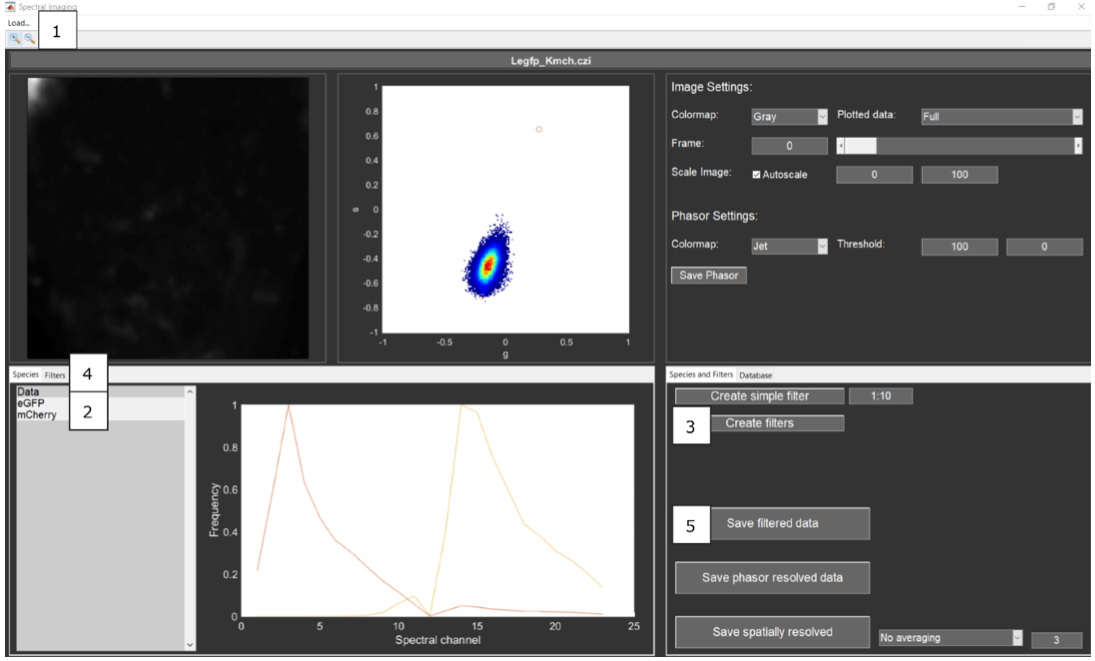
The Spectral User Interface

Select the filters on the Filters tab by pressing the “+” or “right-arrow” key (highlight #4) (the filter’s name will turn green) and pressing the Save filtered data pushbutton (highlight #5). This action creates two .tif files, one weighted towards the green and one towards the red species. Specifically, the signal intensity of each spectral bin of each pixel is multiplied with its corresponding weight, and every weighted pixel is summed up over all spectral bins [Schrimpf2018].

Batch processing is possible via load -> data to database.

The newly generated .tif files contain both the weigthed and unweighted data. They can each be opened and further analysed from the Load… menu of Mia:

Choose the …weighted TIFFs option to select the .tif files per channel. This will display the spectrally weighted data. Mind that the resulting images contain both positive and negative values, this is normal. Choose the …single color TIFFs option to select the .tif files per channel. This displays simply the sum of all spectral channels, and is not so useful.

The original .czi files contain the spectral imaging data. Load the preferred sum of spectral channels into Mia by defining the spectra range in the Options menu. They can each be opened and further analysed from the Load… menu of Mia:

Choose the …Custom data format option to select the original .czi file.

RICS Performance Evaluation

From the menu Open… RICSPE a user interface can be called that allows predicting the optimal RICS image acquisitioning parameters given particular sample properties (concentration, brightness, diffusion constant) [Longfils2019].

References

[Petersen1993]

Petersen, N.O., et al. Quantitation of membrane receptor distributions by image correlation spectroscopy: concept and application. Biophys. J. 65(3), 1135-1146 (1993)

[Wiseman2000]

Wiseman, P.W., et al. Two-photon image correlation spectroscopy and image cross-correlation spectroscopy. J. Microsc. 200, 14–25 (2000)

[Digman2005]

Digman, M.A., et al. Measuring fast dynamics in solutions and cells with a laser scanning microscope. Biophys. J. 89(2), 1317-1327 (2005)

[Digman2009a]

Digman, M.A., et al. Detecting protein complexes in living cells from laser scanning confocal image sequences by the cross correlation raster image spectroscopy method. Biophys. J. 96(2) 96707–716 (2009)

[Toplak2012]

Toplak, T., et al. STICCS reveals matrix-dependent adhesion slipping and gripping in migrating cells. Biophys. J. 103(8), 1672–1682 (2012)

[DiRienzo2013]

Di Rienzo, C., et al. Fast spatiotemporal correlation spectroscopy to determine protein lateral diffusion laws in live cell membranes. Proc. Natl. Acad. Sci. 110(30) 12307-12312 (2013)

[Digman2008]

(1, 2, 3, 4) Digman, M.A., et al. Mapping the number of molecules and brightness in the laser scanning microscope. Biophys. J. 94(6), 2320-2332 (2008)

[Dalal2008]

(1, 2, 3) Dalal, R.B., et al. Determination of particle number and brightness using a laser scanning confocal microscope operating in the analog mode. Microsc. Res. Tech. 71(1) 69-81 (2008)

[Digman2009b]

(1, 2) Digman, M.A., et al. Stoichiometry of molecular complexes at adhesions in living cells. Proc. Natl. Acad. Sci. 106(7), 2170-2175 (2009)

[Hendrix2013]

(1, 2, 3, 4) Hendrix, J., et al. Pulsed interleaved excitation fluctuation imaging. Biophys. J. 105(4) 848-861 (2013)

[Hendrix2015]

(1, 2, 3, 4, 5, 6) Hendrix, J., et al. Live-cell observation of cytosolic HIV-1 assembly onset reveals RNA-interacting Gag oligomers. J Cell Biol 210(4) 629-646 (2015)

[Hendrix2016]

(1, 2, 3) Hendrix, J., et al. Arbitrary-Region Raster Image Correlation Spectroscopy. Biophys. J 111(8) 1785-1796 (2016)

[Schrimpf2018]

(1, 2, 3) Schrimpf, W. et al. Crosstalk-free multicolor RICS using spectral weighting. Methods 140-141:97-111 (2018)

[Longfils2019]

(1, 2) Longfils, M. Raster Image Correlation Spectroscopy Performance Evaluation. Biophys. J 117(10):1900-1914 (2019)