PAM - PIE Analysis with MATLAB
Contents
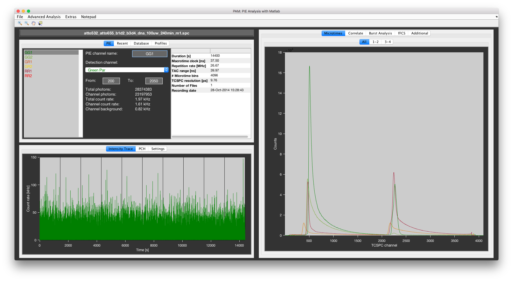
PAM main gui.
Basic functionalities
Loading data
Load data by choosing File -> Load TCSPC data in the menu bar. Currently, PAM supports most TCSPC data file formats. Becker&Hickl hardware is supported for cards of type 130, 140, 150, 630 and 830 (.spc files). PicoQuant hardware is supported for the TimeHarp200, TimeHarp260(N/P), PicoHarp and HydraHarp (.ptu, .ht3, .t3r files). For PicoQuant only the T3 data format is supported because of the data handling in PAM, which is based on separated macro- and microtime information. (The T2 format records photon arrival time with maximum TCSPC resolution in one array, which can be reconstructed from the separate macro- and microtime photon streams in software. We don’t recommend to use this file format, since information is lost compared to the T3 format.)
While PAM is primarily designed for TCSPC data, many of its features (e.g. FCS or image fluctuation analysis) also work with certain non-TCSPC counting or pre-binned data. The way to deal with this type of data is described in more detail in Data structure and Custom file formats.
Standard formats
The following read-in options are always available:
- Single-card B&H SPC files recorded with B&H-Software (.spc):
- This is the general read-in routine for Becker&Hickl (B&H) .spc files. Choose this if you want to load data from a single SPC card.
- Multi-card B&H SPC files recorded with B&H-Software (._m1.spc):
- Use this read-in routine if you are recording data on multiple SPC cards simultaneously. When using multiple SPC cards with the B&H software, the data will be saved in individual files for each card, numbered by the extension _m1.spc, _m2.spc and so forth. Using this read-in routine, select the first .spc file, and all associated files with same name but different number will be loaded.
- PicoQuant universal file format (.ptu):
- PicoQuant’s general time-tagged time-resolved file format, which can be recorded by different hardware. Information about the used hardware is encoded in the file and read out upon loading.
- HydraHarp400 TTTR file (.ht3):
- File format specific to the PicoQuant HydraHarp recorded using the version 2 software.
- TimeHarp200 TTTR file (.t3r):
- File format specific to the TimeHarp200 card from PicoQuant.
- PhotonHDF5 file (.h5):
- Photon HDF5 file as described on http://photon-hdf5.github.io.
- PAM simulation file (.sim):
- Simulated data from PAM’s simulation module.
- PAM photon file (Created by PAM) (.ppf):
- Raw photon data exported from PAM.
- Confocor3 raw files (.raw):
- Raw data files recorded with the Confocor 3 module for Zeiss microscopes.
Custom file formats
The high number of different commercial and custom microscope makes it impossible to accommodate all data and file formats that could be used to analyze data in PAM. An especially big problem is the vast number of different way to encode scanning markers in the data, even when one of the standard TCSPC formats is used. Therefore, we designated a spot in the filetype selection for a custom read-in routine. These routines are stored in the Custom_Read_ins folder in the functions folder and must be matlab function files (.m) of a certain base structure. One of these read-ins can be selected in the profiles tab in PAM and is stored in the UserValues information. This way each lab can create and adjust local read-ins.
The read-in function must have the following function name:
function [Suffix, Description] = MyFunction(FileName, Path, Type, PAM_handle)
The input parameters are:
FileName : A 1 x n cell array containing a string with the filename of each file to be loaded
Path : A string of the folder path of the files
Type : The type must always be 10 and is used to encode the custom read-in information in the FileInfo
PAM_handle : A structure containing all the handles of GUI elements of the PAM main figure. This input does not need to be used in the function, but can be used to query certain setting in PAM.
The output parameters are strings used for the Filterspecs and DialogTitle inputs of the matlab uigetfile function.
The function name should then be followed by a short section like this:
if nargin == 0

    Suffix ='*.mytype';

    Description ='My custom data format (*.mytype)';

    return;

end
This section has the purpose to filter the file selection by a certain file ending and to give a short description of the datatype. Outside of this section the output parameters are not used anymore.
The last requirement of the custom read-in function is to declare some variables global using:
global TcspcData FileInfo
The rest of the code does not have to follow a certain form and can contain other functions or references to non-matlab based functionalities. The only requirement is that the global variables TcspcData and FileInfo have a specific form (described in Data structure).
Data structure
Most data in PAM is stored in the memory as global variables to allow the user easy access to extract the data at any point of the analysis. These variables are:
TcspcData
This variable contains the basic photon information. It is a structure with two fields, MT and MI. Both fields are n x m cell arrays, with n representing the different Tcspc cards or modules used, while m represents the routing information. These cells are addressed by the Detector channels definition of a profile.
Both MT and MI contain entries in these cells for each detected photon.
MT: The macro-time or time since the start of the experiment in clock ticks, stored as a n x 1 double array. In most TCSPC devices the ticks are based on a internal or external clock, of which the period is stored in FileInfo.ClockPeriod. In the case of binned raw data, the clock period should be set to the bin duration and a pseudo-photon entry should be created for each intensity count.
MI: The micro-time or time since last synchronization pulse, stored as a n x 1 uint16 array. If non-TCSPC data is used, these entries should all be set to 1.
FileInfo
This variable contains all the information about the measurement required to perform proper analysis in PAM. It is a structure with the following required field:
FileType : Name of the datatype, needed to determine the correct the read-in routine if the data is to be re-loaded.
Type : Number defining the read-in routine. For custom read-ins the number is always 10.
FileName : Cell containing all the filenames as strings.
Path : Folder path of the loaded files
NumberOfFiles: Represents the number of currently loaded files
MI_Bins : Number of bines used for the micro-time
ClockPeriod : Define the period of the macro-time ticks
SyncPeriod : Defines the period between two laser- or synchronization pulses. Usually identical to the ClockPeriod. Currently not used.
TACRange : Defines the full range of the micro-time. Not always equal to ClockPeriod.
Lines : Number of line of a frame.
Pixels : Number of pixels per line.
MeasurementTime : Total time of the measurement in seconds
ImageTimes : Starting time of each frame in seconds. Has Frames or Frames+1 entries (see ImageStops)
LineTimes : Starting time of each Line in seconds. Is an array of Frames x Lines or Frames x (Lines+1) (see LineStops)
LastPhoton : Arrival time of each photon of a file in clock ticks
ScanFreq : Scanning frequency for line or circular scans.
These fields are always required for PAM to work properly. When data is loaded that does not contain some of the information (e.g. the imaging parameters), they should be initialized to default parameters in the read-in routine.
If both start and stop signals are used for image data, two additional fields are used:
ImageStops : End time of each frame in seconds. If ImageStops is defined, both ImageStops and ImageTimes have Frames entries, otherwise ImageTimes has Frames+1 entries.
LineStops : End time of each line in seconds. If LineStops is defined, both LineStops and LineTimes have Frames x Lines entries, otherwise LineTimes has Frames x (Lines+1) entries.
Additional fields can be created to store information for the user, but they will generally not be used by the program.
PamMeta
This variable contains pre-processed data and other information needed for a fast update of the plots.
UserValues
This variable contains a variety of different settings or other parameters (filepaths, IRF or phasor reference data, etc.) that are not specific to the current file and are stored between sessions. These data are saved in the profile and reloaded upon restart of the program or a change of the used profile.
Setting up a profile
PAM uses profiles to allow the users to work efficiently with data from different setups and configurations. A profile saves the settings of a session on the hard disk, so that the main parameters do not need to be re-entered every time.
Profile management is done in the Profiles tab in the tip-left of the PAM window. To switch to an existing profile, select it in the profiles list and press enter or right click and select Select profile. To create a new profile, right click the profiles list and select Duplicate selected profile or Add new profile. This will prompt the user to enter a name for the new profile. All profiles are stored in the profiles sub-folder of PAM as individual .mat files. When PAM is started, it checks this folder for the profiles list. Thus, profiles can be easily copied to and shared between different computers.
Hint
It is recommended to create a profile for each setup configuration to speed-up analysis of regular experiments.
Note
Switching profiles usually requires the user to reload the data into PAM. It is generally recommended to restart PAM when switching profiles to make sure that all settings are updated.
The two most important settings of a profile are the definitions of the detector and the PIE channels.
Detector channels
Data loaded into PAM is divided into separate channels for the different detectors used. Each channels is associated with an index for the TCSPC card or module (Det# in the detector list) and an index for the routing bit (Rout# in the detector list) used. These values correspond to the indexes of the TcspcData variable, where the corresponding data are stored.
To create a new detector channel, right click the detector list and select Add new microtime channel. The Name, indices and some additional information can be easily changed in the list.
Note
Consistent with the standard MATLAB convention, indexing of the channels/modules/routing starts at 1 and not 0, as with many other programming languages.
Hint
Individual detector channels can be temporarily disabled with the Enabled property in the detector list. For some data types (e.g. the B&H .spc files) this can speed-up data loading and save memory, if only a subset of the detectors is needed.
The individual detector channels are plotted in the Microtime plots and are directly used in some applications (e.g. Phasor referencing).
Defining PIE channels
The majority of applications in PAM do not work directly with the detector channels but rather use PIE channels. A PIE channel contains only photons from a part of the microtime range, thus it is possible to separate the data by excitation (in the case of pulsed interleaved excitation), or use time-gating.
The PIE channels are displayed in the PIE list of the PIE tab in the top-left of PAM. Right clicking the list opens a menu that allows the user to adjust the PIE channels (e.g. creating new channels or deleting existing ones). PIE channels are defined by the detection channel and the microtime range (in units of the microtime bins). The microtime range can be set manually using the edit boxes To and From in units of TAC channels, or interactively by right-clicking the PIE channel and choosing PIE channel -> Manually select microtime range. This will turn the cursor into a crosshair. Select the From and To points by clicking twice into the respective plot in the individual microtime plot tab.
PIE channel notation
Although you can give PIE channels any name you want, we recommend the following notation. Since the idea of PIE channels is to separate photons by detection color and excitation source, this information should be encoded in the given PIE channel name. Choose a single letter to encode the color (e.g. G for green, R for red, B for blue, Y for yellow) and use the single letter code to denote excitation and detection color in this order (e.g GR, BY, BR).
For example, if excitation was performed using a 532 nm laser (green, G), and the photons are detected in the red spectral region (red, R), the PIE channel for red photons after green excitation should be given the name GR. If additionally polarized detection was used, append a number to encode this information (1 for parallel polarization, 2 for perpendicular polarization).
Note
A typical PIE-MFD setup with two color excitation and two color polarized detection will thus have the following PIE channels: GG1, GG2, GR1, GR2, RR1 and RR2.
Combined PIE channels
In some cases it might be useful to pool data from multiple detectors (e.g. combine polarizations). Since each PIE channel is associated with only a single detector channel, this requires combined PIE channels. To create a combined PIE channel, select the individual ones, right click the PIE channel list and select PIE channel -> Create combined channel. The new channel will refer back to its parents, so that changes (e.g. of the microtime range) will be automatically updated.
Note
A combined channel uses the position of its parents in the list as reference. Deleting channels might thus disrupt the references. Therefore, combined channels should be re-defined whenever any changes were done to the PIE channel list.
Note
Most applications in PAM will treat combined channels just as any other channel. However, some functions (burst search, lifetime fitting and filtered FCS) require standard PIE channels to work.
Saving the meta data
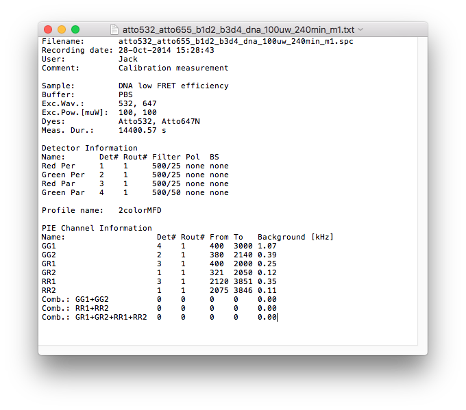
An example meta data file.
To save meta data associated with your measurement, enter the respective information into the table in the Profiles tab. Click Save Metadata to store the meta data in a .txt. file with the same name as the loaded file in the respective folder.
In addition to the user specified information from the meta data table, the recording date and measurement duration are stored together with the information from the detection channel table and the PIE channel definitions including the stored background count rates.
Data exploration
Several standard plots of the raw data are available to investigate the data set. Microtime histograms are plotted on the right side. On demand, a intensity trace, photon counting histogram or image can be plotted. Disable/enable these plots in the Settings tab using the respective checkboxes.
Hint
Disabling the calculation of intensity trace, photon counting histogram and/or image will significantly speed up the loading of data, especially for large data sets. Re-enabling the plots after the data has been loaded will still provide you with the plots on-demand.
Microtime plots
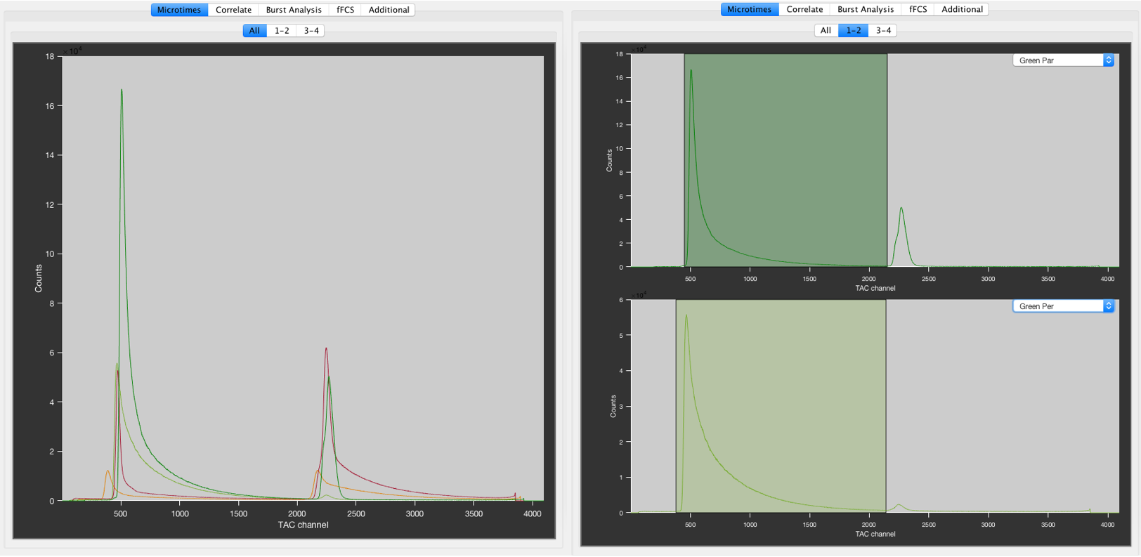
The All microtime tab (left) and the individual microtime tab (right). The settings are 2 tabs and 2 plots per tab. The first tab 1-2 shows the two green detection channels, the second tab 3-4 shows the two red detection channels. The green shaded areas indicate the defined PIE channels on the green detection channels.
The microtime histograms of the defined detection channels are plotted on the right. The All tab show all microtime histograms in a single plot.
The individual plots can be customized using the settings in the Settings tab in the bottom left of PAM. Choose the number of tabs and the number of plots per tab, then define the detection channel for each plot using the dropdown menu in the top left of the respective plot.
PIE channels will be shown as shaded areas in the respective PIE channel color. You can directly click the individual microtime plots to define the microtime range of the PIE channels as described in Defining PIE channels.
The x-axis unit for the microtime histogram can be changed between TAC channels and time in nanoseconds using the checkbox in the Settings tab.
Right-clicking the plots allows switching between log and lin scales, and allows showing/hiding the scatter and IRF data.
Intensity Trace
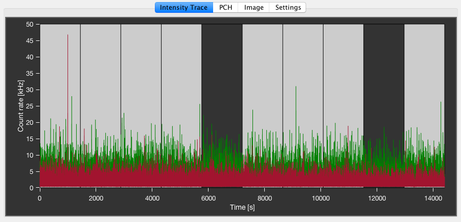
Example time trace of two PIE channels with unselected macrotime blocks (dark blocks).
The Intensity Trace tab shows the intensity time trace for the selected PIE channel(s). The binning of the signal trace can be changed in the Settings tab.
For FCS analysis, the measurement can be split up into several blocks of equal size. To select/unselect a certain time range, left-click on the respective block, turning it dark. This will exclude it from FCS analysis. A second left-click will re-enable the block. In the Settings tab, one can change how the blocks are defined using the Macrotime sectioning type dropdown menu. Constant time will split the measurement using a constant time interval per block, specified by the value for the Sectioning time in seconds. Constant number will split the measurement into a number of blocks specified by the Section number, adjust the time per block based on the measurement duration.
Photon counting histogram
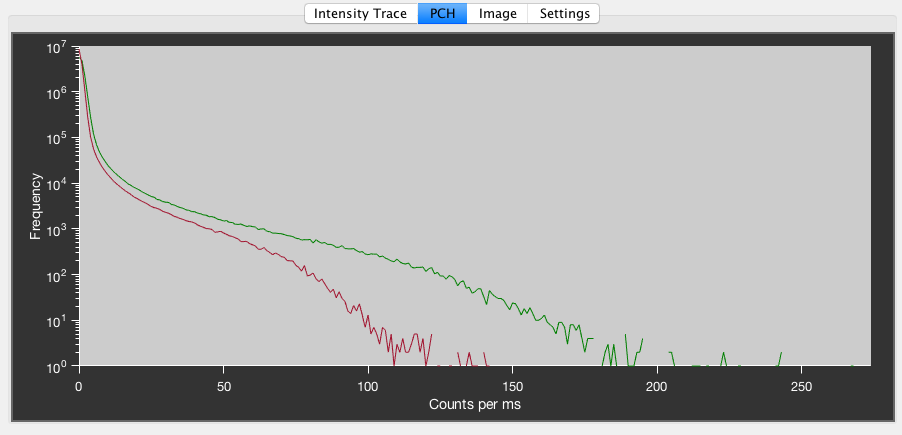
Example photon counting histogram of a dilute solution. The peak at low photon counts is background noise, while the tail towards higher photon counts originates from the fluorescent molecules.
The PCH tab show a histogram of the photon counts per millisecond for the selected PIE channel(s). It can be useful to identify bright particles like aggregates in the solution. Fitting of photon counting histograms as described in [Chen1999] is currently not implemented in PAM.
Image
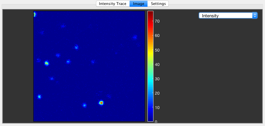
The Image tab.
If the data has the required information to be processed into an image (i.e. pixel/line/frame markers), a raw image of the selected PIE channel can be shown in the Image tab. In addition to the intensity image, a lifetime image based on the mean microtime can be calculated by checking the respective checkbox in the Settings tab. Switch between intensity and lifetime image using the dropdown menu in the Image tab.
Hint
The scaling and colormap of the image can be adjusted with the matlab colormap editor by right clicking the colorbar. Click on the image once before adjusting to make sure that the image is the active axes.
Exporting raw data
The data of each PIE channel can also be exported, either to the matlab main workspace or saved as a standard file format (e.g. TIFF or Text). To do that, select the PIE channels to be exported in the PIE channel list and right click to and choose the Export… menu. There are different exporting options available:
…Raw data (total): Copies the raw photon data of the PIE channels to the main workspace.
…Raw data (per file): Copies the raw photon data of the PIE channels to the main workspace, separated by the individual files loaded.
…image (total): Opens a new figure displaying a summed up images and copies the intensity data to the main workspace.
…image (per frame): Copies the intensity data per frame to the main workspace as 3D arrays.
…image (as .tif): Saves the 3D image stack as a TIFF in the selected folder with the name of the first file and the PIE channel as appendix.
…microtime pattern (as .dec): Save the microtime histogram data as a .dec file for loading into the lifetime analysis sub-program. The .dec file are simply text files.
A more advanced method of exporting PIE channel based images is described in Batch analysis.
IRF and background/scatter
Per PIE channel, the ‘instrument response function’ (IRF) pattern and the scatter pattern are needed to perform reconvolution lifetime analyses in TauFit, Burst Analysis, the average background count rate is needed to correct burst data. Sharp data such as the IRF is additionally needed to carry out Detector calibration.
Recording the IRF:
- Some dyes with a long lifetime can be quenched to an IRF by using a saturated solution of potassium iodide (KI), for example ATTO488 or ATTO655. Always prepare the KI solution fresh, or store it aliquoted in the freezer. Avoid KI crystals by spinning down the tube and pipetting only the supernatant onto the coverslip. Add concentrated dye to the KI solution to achieve the needed signal intensity at the laser power normally used. If necessary, increase or decrease the laser power. Focus far enough from the coverslip to be sure to record at constant intensity.
- Scattering of water (only works if the emission filter transmits a bit of excitation light). Reflection of laser light on a glass coverslip is not a good idea, as the glass might contribute to background signal with a lifetime.
- Removing the emission filter and recording laser reflections. Be careful not to damage your detectors!!!
- A dye with an intrinsically short lifetime (malachite green, bengal roze), although these typically look a bit different than the actual IRF.
Before storing the IRF pattern, consider using it to check possible count rate dependent shifting of the used detector(s).
- Recording the scatter pattern / background:
- Record a measurement of the buffer, accounting for any impurities that might be present in the sample.
- Storing the IRF pattern:
- To store the IRF pattern for all PIE channels in the Profile from a single IRF measurement, load the measurement into PAM and select File -> Store loaded data as IRF (for all PIE channels). This will save the microtime pattern of the currently loaded data for all PIE channels as the associated IRF pattern. To store the IRF for individual PIE channels, instead right-click the PIE channel that you want to set the IRF for and select Save IRF for the selected PIE channel.
- Storing the scatter pattern / background:
- Load the measurement and select File -> Store loaded data as Scatter/Background. This will save the microtime pattern of the currently loaded data for all PIE channels as the associated background/scatter pattern and store the count rates of the individual PIE channels as the background count rates.
You can display the currently stored IRF and background patterns in the microtime plots by right-clicking the microtime plot and selecting Plot IRF or Plot Scatter Pattern.
Using parallel processing
Parallel processing using multiple cores of the CPU based on MATLAB parfor loops is currently implemented for the computation of correlation functions, 2CDE filter calculation, burstwise lifetime fitting and simulation of photon data. When using this feature, consider that it takes some time to set up the parallel pool (~1 minute). You can enable this feature using the menu Extras -> Parallel Processing -> Enable Multicore. The number of cores can be defined using the Number of cores option. Consider using less cores than physically available if you want to perform other tasks while the analysis runs.
Fluorescence Correlation Spectroscopy
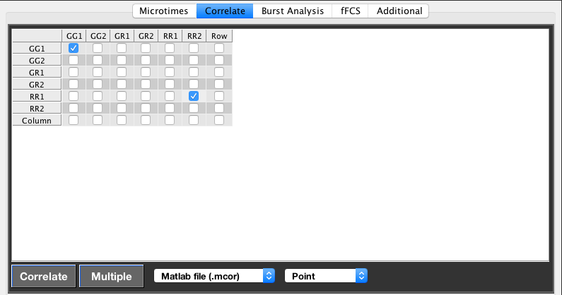
The current selection will calculate the autocorrelation of channel GG1 and the cross-correlation between the channels RR1 and RR2.
Calculation of fluorescence correlation functions is performed on the basis of the defined PIE channels using the correlation grid in the GUI. Autocorrelation functions fall on the diagonal line, while cross-correlation functions are performed by checking off-diagonal elements. Usage of the last row or column will select all elements in the respective row/column. Clicking the bottom right checkbox will select all auto-correlations.
Correlation functions are calculated in one direction in time, delaying the column channel \(I_2(t+\tau)\) with respect to the row channel \(I_1(t)\):
Here, \(<>\) denotes time averaging over the measurement. Temporal auto- and cross-correlation curves are calculate based on a multiple-tau correlation algorithm (see [Felekyan2005] for details). The time axis follows a multiple-tau scheme, doubling the time interval every 20 steps in units of the smallest available time difference given by the macrotime clock of the measurement. (The time delay axis is thus given by [1,2,3….,18,19,20,22,24,…36,38,40,44,48,…] and so forth.)
Clicking Correlate will perform the chosen correlation for the currently loaded file. Fitting of the correlation functions is performed in FCSFit or Pair correlation analysis, depending on the data type.
Multiple files can be correlated in one step by clicking the Multiple button. Select multiple files to be correlated using the open-file dialog. All files will be treated as currently defined.
Correlation functions are generally saved in a MATLAB file format (.mcor), allowing the data to be easily loaded into the MATLAB workspace again. Alternatively, the correlation results can be saved in a general text file (.cor) for processing in other software. Both save formats can also be chosen simultaneously. Choose the output format using the left popup menu.
The user can choose to coarse-grain the time axis by applying a Divider, available via right-click on the correlation grid. This divider effectively reduces the maximum achievable time resolution by the specified factor. If, for example, a clock tick is 100 ns and a divider of 10 is specified, the earliest time bin will span 1 \(\mu\textrm{s}\). This divider might be useful when the laser repetition does not match the macrotime clock (e.g. laser only pulses every n th clock tick).
PAM currently implements five correlation methods which can be chosen using the right popup menu.
Point-FCS
Choose Point if you only want to calculate the temporal correlation function of the photon trace. Individual correlation functions are determined for each macrotime block (see intensity trace plot), which are used to address the error in the correlation function by calculating the standard error of the mean as:
where \(\sigma\) is the standard deviation and N is the number of macrotime blocks.
It may be of interest to exclude certain time intervals from the calculation of the correlation function (e.g. if large aggregates traversed the focus). This can be achieved before the calculation by unchecking the respective macrotime block, or after the calculation by clicking the respective correlation function in the preview plot. Selected curves are shown as solid lines, while unselected curves are plotted as dashed lines.
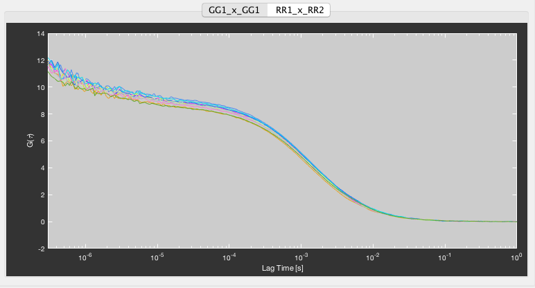
The correlation preview window.
By default, all calculated curves are saved in the results file, so no further action is required if no curve is to be excluded. If a selection is made, confirm it by right-clicking the plot and choosing Save selected correlations. The right-click menu additionally allows to select or unselect all curves at once.
Suppression of afterpulsing
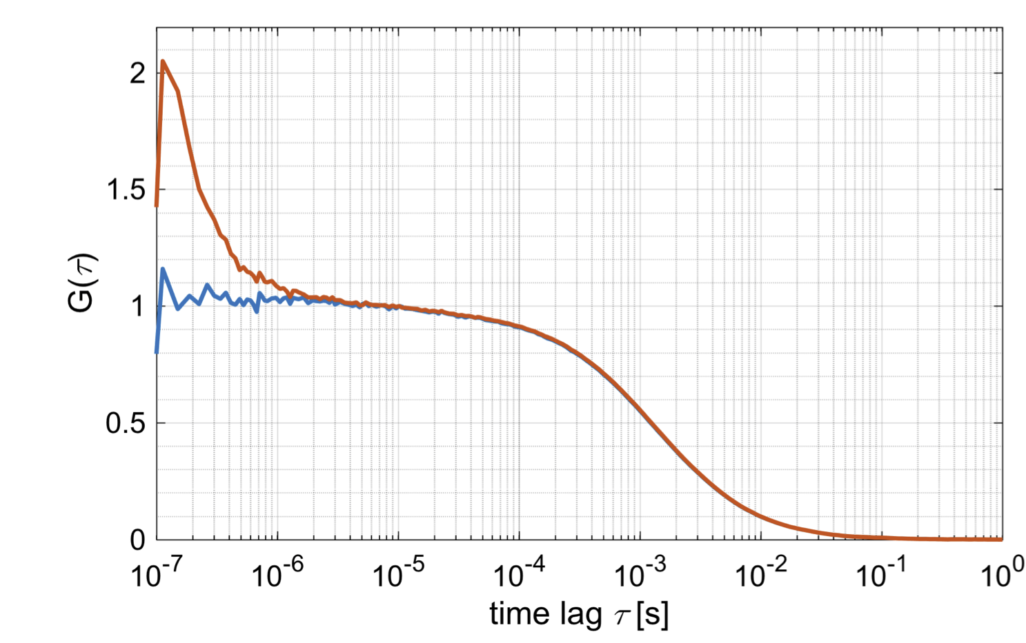
Removal of afterpulsing by fluorescence lifetime correlation spectroscopy. Red: no correction, blue: corrected.
For autocorrelation analysis, detector afterpulsing can be filtered by selecting the Correct for afterpulsing checkbox. This will apply a flat background correction using FLCS to suppress the effect of afterpulsing of signal recorded on a single detector. See [Enderlein2005] for details.
Removal of aggregates
FCS measurements are prone to artifacts cause by large aggregates. Since the contribution of species scales with the square of the brightness, single large aggregates can dominate the correlation function.
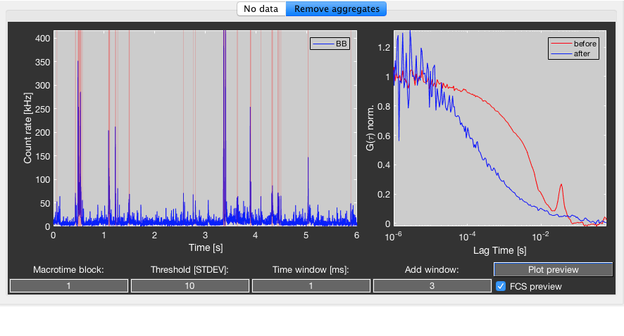
Use the Remove aggregates tab to preview the parameters for the removal of aggregates. The algorithm will perform a burst search by using a sliding time window, which will identify signal spikes (see here for more details). The count rate threshold that has to be exceeded is specified in units of the signal standard deviation. Tune the size of the time window depending on the diffusion time of the aggregates that should be excluded. Additionally, you can add a time window around the edges of detected spikes to further stretch out the regions where aggregates are detected. The algorithm will erase the spike region and fill them with random Poissonian noise.
Choose the macrotime block (based on the sectioning of the measurement) you want to preview and click the Plot preview button. This will display the signal trace binned using the specified time window and highlight excluded time regions by red shading. Check the FCS Preview checkbox to also get a preview of the uncorrected FCS curve (red) and the corrected FCS curve (blue). If multiple autocorrelations are selected in the correlation table, only the first selection is displayed in the preview module.
Check the Remove aggregates checkbox under the correlation table to enable filtering using the specified criteria for the FCS calculation.
Note
Afterpulsing correction and aggregate removal are exclusive and can not be combined.
Nanosecond-FCS
Nanosecond-FCS (or full-FCS) uses the microtime information in addition to the macrotime information to reconstruct the photon arrival time with highest time resolution (given by the resolution of the photon microtime), by:
\[t_i = \textrm{MT}_i \cdot \textrm{TAC} + \textrm{MI}_i\]
Here, TAC is the TAC range, MT is the macrotime and MI is the microtime.
Two modes are available for nanosecond-FCS. Microtime will perform the correlation using a multiple-tau time axis as used for point-FCS, while Microtime (linear) will instead use a linear time axis from -10 \(\mu\textrm{s}\) to 10 \(\mu\textrm{s}\) with a resolution of 100 ps, based on the interphoton time distribution as described in [Nettels2007].
Pair correlation function
Fluorescence pair correlation analyzes the temporal fluorescence correlation spatially resolved for scanning data. If a certain pattern was repeatedly scanned with a constant frequency, the data will show a direct relationship between the measurement time and position. PAM uses this relationship to divide the photons by position, by separating them into (temporally) equally sized bins, defined by the #Bins parameter and the scanning frequency (FileInfo.ScanFreq).
Note
For continuous scanner movement, the number of bins should be chosen such, that the focus movement during the bin duration is significantly smaller than the focus size, generally <50nm. If scanning was discontinuous (i.e. the focus jumps between positions and stays there), the number of bins should be equal to the number of scanned positions, or a multiple of that, if the distance between positions is very small.
Each bin now only contains photons that originates from a particular focus position. Since the data now have temporal gaps, the timing for the correlation algorithm is reduced to the scanning frequency. Thus, the temporal resolution of the correlation functions is determined by the scanning frequency and not the sampling speed.
For each spatial bin, a temporal auto-correlation is calculated. Additionally, temporal cross-correlations between different bins and for different spatial lags are calculated. In most cases, not all spatial lags are needed for analysis, e.g. for very large distances, the correlation amplitudes are too low to be properly analyzed. For such cases, the user can limit the spatial lag range to be calculated, by using the Distance field and standard matlab vector indexing (e.g. 1:50 or [9,10,12], etc.), thus reducing the calculation time. The individual calculations are performed with the same algorithm as normal FCS.
Note
The terms used in the case of pair correlation refer to the spatial auto- and cross correlations. But pair correlation also works for correlating signals from different channels (e.g. color or polarization). That means, it is possible to calculate spatial and spectral cross-correlations. The same selection of PIE channels as in standard FCS is used.
The pair correlation data is save a matlab bases .pcor format and can be easily loaded into the matlab main workspace or analysed with Pair correlation analysis.
FLCS/fFCS
Fluorescence lifetime correlation spectroscopy and filtered-FCS use differences in fluorescence lifetime or anisotropy to separate species in a mixture by assigning statistical weights to photon based on the microtime ([Boehmer2002] and [Felekyan2012]).
The basic assumption of FLCS/fFCS is that the microtime pattern of the measured mixture can be expressed as a linear combination of the microtime signatures of the individual species. One can define statistical filters from the linear decomposition which are used to assign weights to the individual photons based on their microtime.
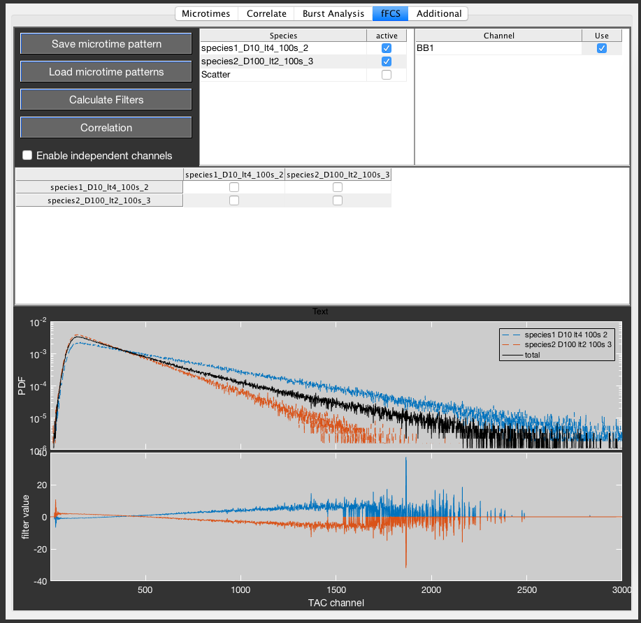
The FLCS/fFCS GUI.
To perform fFCS analysis, the microtime patterns of the pure species need to be known. The current implementation assumes that a pure measurement of the components is available, or that they can be extracted from a single-molecule measurement. If the pure components are available, load the individual measurements and save the respective microtime pattern using the Save microtime pattern button. This will save all the microtime information in a .mi file.
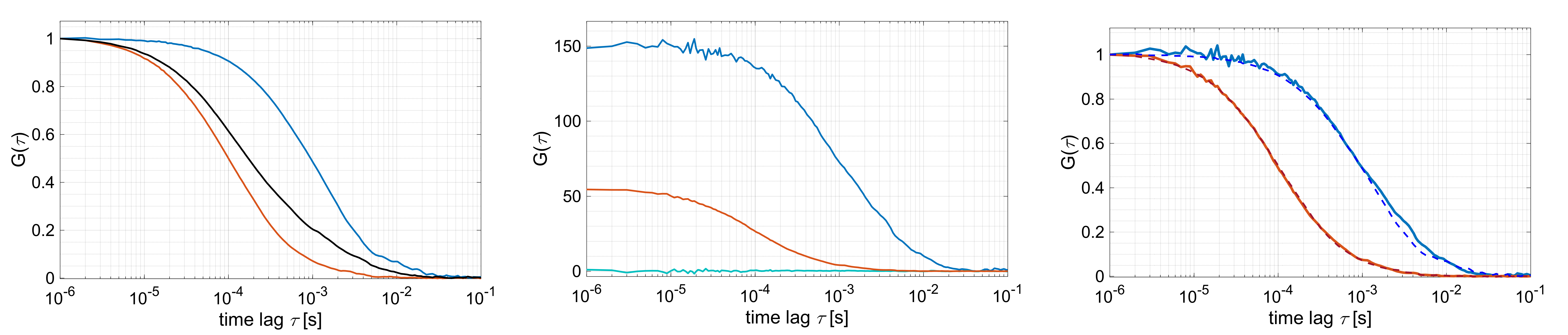
Example FLCS analysis of two species with different diffusion coefficient and fluorescence lifetime (2 ns and 4 ns). (Left) Pure autocorrelation functions of fast diffusing species (red, lifetime of 2 ns), slow diffusing species (blue, lifetime of 4 ns) and a 2:1 mixture of fast and slow species. (Middle) Filtered species auto- and cross-correlation functions using the filters shown in the previous figure. (Right) Comparison of filtered auto-correlation functions from the mixture (solid lines) and the pure autocorrelation functions of the individual species (dashed lines).
Load the individual microtime patterns (.mi files) into PAM using the Load microtime patterns button. This will add the respective species to the Species table. Select the species to consider in the Species list. A Scatter species is always available based on the stored scatter pattern. PIE channel that are defined in all loaded .mi files will be listed in the Channel list. Select which PIE channels to use for filter generation. If multiple PIE channels are selected, the microtime histograms will be stacked for the global filter generation. Press the Calculate Filters button to generate the filters for the selected species.
Use the Correlation table to select which auto- and crosscorrelations are to be performed and press the Correlation button to perform the correlation.
Check the Enable independent channels checkbox to use two independent channels that can be crosscorrelated. This will allow to assign PIE channels to two independent channels. Filters will be independently generated for both channels and used in the crosscorrelation between the channels. Use this option to circumvent detector dead time and afterpulsing artifacts at sub-microsecond timescales by crosscorrelating signal detected on independent detectors.
Burst Analysis
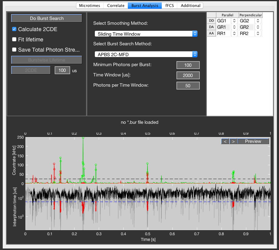
BurstSearch tab overview.
The Burst Analysis tab is used to extract single-molecule events from a PIE-MFD measurement. Different burst search methods are available, whose parameters should be adjusted for the specific measurement at hand. PAM calculates basic burst wise parameters like FRET efficiency and labeling stoichiometry automatically, while additional parameters (fluorescence lifetime, ALEX 2CDE filter…) can be calculated on demand.
Burst search methods and burst selection
Burst search methods are categorized by experiment type (two color, three color, polarized detection used or not) and by burst selection method (APBS, all photon burst search, or DCBS, dual channel burst search, [Nir2006]). Two color or three color experiments are denoted by 2C or 3C, respectively. The use of polarized detection is signified by appending the tag MFD or noMFD.
Burst selection
The general burst selection method is the all photon burst search (APBS), which disregards the channel information and combines all photons into a single signal trace on which the burst search is performed. This way, single and double labeled molecules are detected likewise. This is the general setting that should be applied to unknown systems.
Dual channel burst search (DCBS) performs APBS burst searches on the signal trace after donor excitation (GG + GR) and after acceptor excitation (RR) separately. Only time intervals during which the two separate burst searches identified a burst are kept. This has some consequences for how different events are recorded. Firstly, donor and acceptor only events will not be detected. Secondly, bursts which show photobleaching of either donor or acceptor fluorophore will be truncated. Thirdly, blinking events of either donor or acceptor fluorophore will segment the single molecule event. DCBS is effective in limiting the analysis to only double labeled molecules.
Tip
Always start analyzing data with an APBS, to get an idea about the system and to look for possible artifacts (impurities, high amount of photobleaching) and to determine correction factors from the donor and acceptor only subpopulations (see BurstBrowser). Use DCBS when the system at hand is characterized and a quick analysis of the relevant double labeled molecules is desired.
Warning
When using DCBS only, be cautious of low FRET populations! If no double labeled molecules are present in solution, DCBS will still find multi-molecule events, which will have a low FRET efficiency. Look at the APBS to ensure that the detected low FRET species is indeed a population and not just a bridge between acceptor and donor only populations.
Smoothing and burst search methods
There are currently two different methods to smooth the signal trace and to perform burst thresholding.
- Sliding time window:
This method uses a sliding time window centered around each photon to estimate the local count rate. If the local count rate exceeds the threshold, the center photon is assigned to belong to a burst. If a certain number of consecutive photons pass the threshold, they are grouped into a burst. See [Nir2006] for more details. The user can specify the time window width in microseconds, the required photons per time window, and the minimum number of photons per burst. The time window T is symmetrically centered, i.e. ranging from t-T/2 to t+T/2.
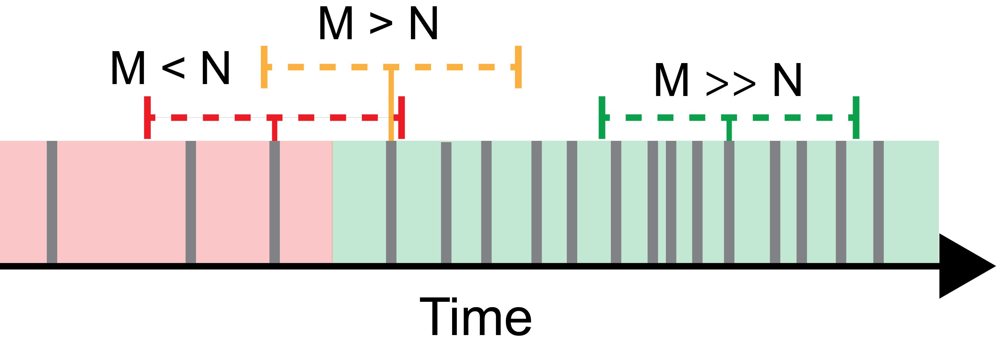
Illustration of the sliding time window burst search. N is the threshold number of photons per time window and M is the actual number of photons in the illustrated time window. Individual photon arrival times are indicated by grey bars.
- Interphoton Time with Lee Filter:
- This method selects bursts based on a threshold on the interphoton time, which will be short during a burst of photons compared to long interphoton times during background signal.The interphoton time trace is smoothed using a Lee filter, which has the property to smooth regions of constant signal, while leaving regions with rapid parameter changes (i.e. the edges of bursts) untouched. The user can specify the minimum number of photons in a burst, the size of the smoothing window in one direction N, and the interphoton time threshold in microseconds (lower values correspond to higher count rates). The smoothing window parameter N corresponds to a total number 2N+1 photons considered for the smoothing, centered around the respective photon. The smoothing parameter \(\sigma_0\), which characterizes the noise standard deviation, is estimated by the global standard deviation of the interphoton times. For more information, see [Schaffer1999] and [Enderlein1997].
Burst search preview
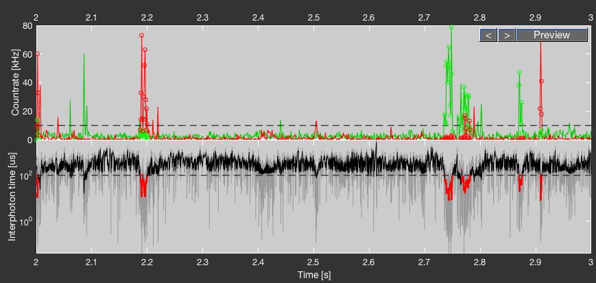
The burst search preview window.
To judge the chosen parameters, a preview window is displayed in the bottom part of the Burst Analysis tab. Click the Preview button to update the preview display, and use the arrow buttons to go forward and backward in time by one second.
The top plot shows the intensity traces after donor excitation (GG + GR, green) and after acceptor excitation (RR, red) using a time bin of 1 ms. The dashed line shows the count rate threshold given by the burst search parameters. For Sliding Time Window it is given by the number of photons per time window divided by the time window length, whereas for Interphoton Time with Lee Filter it is given by the inverse of the interphoton time threshold. Time bins that belong to an identified burst are indicated by colored open circles.
The bottom plot shows the raw interphoton time trace in grey, together with the smoothed trace in black. The interphoton time threshold is shown by the dashed line. Photons that belong to a burst are colored red. If Sliding Time Window is selected, a default smoothing window of 30 is used for display, and the interphoton time threshold is given by the inverse of the count rate threshold.
Note
Depending on which burst search method is chosen, primarily use the respective plot (top for Sliding Time Window, bottom for Interphoton Time) to evaluate the burst search parameters. The respective other plot is just shown for illustrative purposes.
PIE channel assignment
The next step after choosing the experiment type and burst search method is to correctly assign PIE channel to FRET channels. If the standard PIE channel notation has been used (see PIE channel notation), this step is straight-forward. In the Burst Analysis interface, FRET channels are defined using the same notation as for PIE channels, with the more general notation of D for FRET donor and A for FRET acceptor. The FRET channels are thus DD, DA, and AA, each defined per detection polarization. Use the drop-down menu to select a PIE channel for each FRET channel. (For three-color FRET, the assignment table will instead denote channels by color as used for PIE channel definition, i.e. BB, BG, … etc.).
Note
It is not possible to change the photon assignment (i.e. the properties of the PIE channels) after the burst analysis has been performed.
Tip
Take the time to again check the detector assignment and microtime boundaries of the individual PIE channels. Common errors are the wrong assignment of parallel and perpendicular channels, and wrong microtime ranges that lead to false assignment of photons (e.g. because the timing of the hardware was changed).
Performing the burst search
Once all parameters have been set, start the burst analysis by clicking Do Burst Search. Once the burst analysis is finished, it will create a subfolder in the location of the raw data with the name given by the raw data file. The burst data is stored in a file with the .bur ending. The name of the file is given by the file name of the raw data with appended burst search method. Raw photon data is saved in a separate file with ending .bps (for ‘burst photon stream’) to avoid having to reload the original data. Additionally, the specified burst search parameters as well as all other available meta data (see Meta data saving) is saved in a .txt file with the same name.
Additional burst wise parameters
After the burst search is performed, two more parameters can be determined: the fluorescence lifetime and the two-channel kernel density estimate filter. After the burst search, the respective buttons labels are red to indicate that the parameters have not been determined. After calculation the button labels turn green.
Burstwise fluorescence lifetime
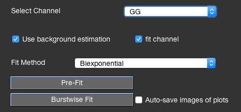
Changed settings windows when calling TauFit for burstwise lifetime determination.
Click Burstwise Lifetime to open an instance of TauFit. The program structure is the same as described in the TauFit documentation. The main plot shows the cumulative microtime histograms of all selected bursts. Align the microtime channels as described in the TauFit documentation. The quality of the alignment can be judged using the Pre-Fit button, using a single or biexponential fit model. Use the popup menu to go through all colors (GG and RR for two-color experiments, BB additionally for three-color) to align all color channels and ensure the right correction factors are used. Click Burstwise Fit to start the lifetime fit.
Note
The donor decay usually shows multiexponential behavior (donor only molecules and one or more FRET species). Use the biexponential fit model to judge the correctness of the microtime shift parameters (most crucial is the IRF shift). The acceptor decay usually shows a monoexponential decay, so a single exponential is sufficient.
Uncheck the fit channel checkbox if you do not want to fit the lifetime for this channel. The Auto-save images of plots automatically saves pictures of the performed alignment and pre-fits so you can inspect it later to ensure the lifetime has been determined correctly.
The lifetime fitting is performed using a single exponential model function and is based on a maximum likelihood estimator as described in [Maus2001]. If the Use background estimation checkbox is enabled, a scatter contribution using the microtime pattern of the specified scatter measurements (i.e. of the used buffer) is added with a fixed fraction \(f_\textrm{BG}\), estimated based on the total signal in the burst S, the background count rate BG and the burst duration T:
Two-channel kernel density estimate filter
Additionally, the two-channel kernel density estimate filter (2CDE) as described in [Tomov2012] can be calculated by clicking the 2CDE button. The calculation is based on a single variable parameter, which is the time window to estimate the photon density. This parameter should be larger than the average interphoton time, but smaller than the burst length. Generally, a value of 100 \(\mu\textrm{s}\) yields good results. 2CDE filter calculation supports the usage of multiple cores.
Correlation analysis with time window (purified-FCS)
If you want to perform a correlation analysis on a subset of bursts with the option of adding a time window around the burst to correctly determine the diffusion time of molecules, it is required to check the Save total photon stream checkbox. It is currently not possible to re-access raw data to perform this step at a later time point, so when correlation analysis is to be performed, the decision has to be made at the time point of the analysis. The total photon stream is saved as an .aps file. See Burstwise FCS for more information on using a time window in burstwise FCS.
Note
The resulting .aps file will be of similar size as the raw photon file. Be aware of this when disk space is a concern.
Using a total measurement for photon distribution analysis
Photon distribution analysis (PDA) can be performed on the total photon stream. To export the total measurement to PDAFit, right-click the Do Burst Search button and select Export total measurement to PDA. This will chop up the data into time bins of 1 ms. Currently, this option is only available for two-color MFD data.
Phasor referencing
The Phasor Referencing tab is used to convert the raw photon data into referenced phasor FLIM data to be analyzed with Phasor Analysis sub-program. The processed data is saved as a .phr file that is based on the standard .mat matlab data format and can be easily loaded into the matlab command window.
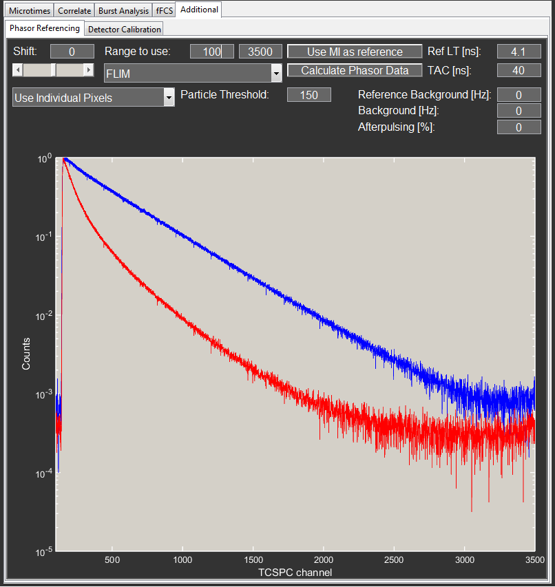
Reference data and settings
To account for the IRF of the system, a reference file of known mono-exponential lifetime is needed (an IRF measurement with a lifetime of 0 also works) for all calculations. During referencing, the program calculates the raw phasor of the reference and compares it to the expected values (based on the reference lifetime set with the corresponding editbox). The parameters (phase and modulation) needed to move the measured to the expected values represent the influence of the instrument and are then applied to the actual measurement to remove the bias from the IRF.
A phasor plot depends on the underlying frequency. PAM uses the full range of the microtime histogram as the period of this frequency.
The reference histogram is stored in the UserValues information of the current profile with the Use MI as reference button and is displayed in blue in the phasor histogram plot.
Note
The phasor referencing works on the full detector channel and not just the PIE-channel. The current detector channel can be selected with the corresponding popup-menu.
Background corrections
Uncorrelated stray light and detector dark-counts result in an additional (infinite) lifetime component for the phasor calculations. Since the extent of the background influence depends on the total signal, it has to be corrected individually for each pixel. In PAM the user can set a background count rate for both the reference and the measurement files. Additionally, an afterpulsing probability can be set to further correct the signal.
Note
In most cases afterpulsing affects the reference and the measurement data to the same extent and thus is removed automatically in the referencing procedure. This is however no longer the case if the used range is restricted. In practice, for high enough signals (SNR>100) no corrections are necessary.
Note
Background originating from the sample, most commonly cell auto-fluorescence, has usually an unknown lifetime and cannot be removed during the referencing. Its influence has to be considered during data interpretation.
IRF shift and artifacts
Some detectors (mostly APDs) used for FLIM applications show shifts of the IRF based on the signal intensity and other environmental effects. In PAM, fast, count-rate dependent influences can be removed during data loading (see Detector calibration). To correct for very slow changes (on timescales longer than a measurement), the user can shift the reference relative to the measurement histogram with the corresponding editbox or slider.
Certain regions of the microtime range can contain artifacts that strongly influence the phasor calculations. A common sources for such artifacts is spectral cross-talk in multi-color PIE experiments. If these artifacts are sufficiently separated in time from the actual signal, they can be simply removed by limiting the Range to use. To limit the effect of this cutting, the remaining range should be at least a factor of 5 longer than the longes relevant lifetime component (usually >25ns per color or repetition rates <40MHz).
Note
The phasor frequency is no affected by the used range, bins outside of the range are simply set to 0. Thus, experiments with different ranges (e.g. singe and multi-color experiments) can be compared, as long as artifacts from cutting can be neglected and the microtime ranges are the same.
Phasor calculation
Once all relevant parameters are set, the phasor data for the currently loaded data can be calculated and saved by clicking on the Calculate Phasor Data. Hereby, all frames and files are added, resulting in a single phasor frame. Most of the calculation is performed using C++ to decrease the calculation time.
Particle detection
Usually, a phasor is calculated for each pixel individually. However, in some cases it might be useful to pool several pixels for the calculation to increase the signal-to-noise or decrease measurement time. This is especially useful when an average phasor of individual well-separated particles or cells is desired. For such cases, a Particle detection module is currently in development. To generate the correct input type for this, switch from Use Single Frame to Framewise Phasor and calculate the phasor as usual. This saves the data as a normal, summed up .phr file for standard phasor analysis and also as a .phf file that contains the information for each frame and pixel and can be loaded with the Particle detection) module.
Detector calibration
Avalanche photodiodes used for single-photon counting often show a count rate dependent shift of the instrument response function. In our experience, the COUNT modules from LaserComponents are affected more strongly than the commonly used SPCM modules from Perkin Elmer (see [Otosu2013]). However, if the effect is accounted for, COUNT detectors have a superior IRF. The degree of this effect varies on a module-by-module basis, and has thus to be calibrated for every detector individually. For Perkin Elmer APDs (and maybe others) some other artifacts occur that cannot be easily corrected for.
Before attempting to correct data, first verify whether your detector shows a count rate dependent IRF shift. We find it simplest to either record images with highly varying count rates (e.g. a mixture of dimly and brightly fluorescent cells), or to record a time trace where the laser power is modulated between high and low. If no obvious artifacts appear in the experimental decay, the detector likely does not require any correction.
To be able to clearly identify a possible correlation between the photon arrival (micro-)time and the (macro-)time between photons, and to sample long, but also short interphoton times enough, it’s best to avoid a large spread on the photon arrival time. Therefore, only use high intensity IRF data (~100 kHz) recorded for 5-10 min to have >30 million photons.
To compute the calibration curve, photons are sorted based on the macrotime difference to the previous photon, and microtime histograms are calculated for the sampled interphoton times. The peak positions of the microtime histograms are extracted to calculate the IRF shift with respect to the IRF at long interphoton times.
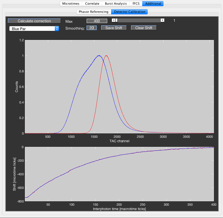
The detector calibration GUI.
To determine the detector calibration, load a measurement and select the detection channel using the dropdown menu. Select the range of interphoton times in units of the macrotime clock that should be calculated (the range should extend to at least 20 \(\mu\textrm{s}\)). Click Calculate correction to compute the calibration.
The top plot shows the uncorrected (blue) and corrected (red) microtime histogram. Using the slider in the top right, one can examine the individual uncorrected microtime histograms for the selected interphoton time (plotted in green). The bottom plot shows the calculated correction lookup table in red. If a smoothing larger 1 is selected using the edit box, the smoothed correction curve is shown in blue. Smoothing is performed using a simple moving average filter of specified size.
Save the shift using the Save Shift button. If a previous calibration is stored, clear it first using the Clear Shift button. The correction is applied on read-in of the raw data, so the current data has to be reloaded for the correction to be applied.
You can export the current detector calibration using File -> Load/Save Calibrations… -> Save Detector Shifts to File to a .sh file. Reload stored detector shifts using Load Detector Shifts. This will overwrite currently stored detector calibrations in the profile.
Note
The calibration is defined based on units of the macrotime clock and specific to the used TCPSC resolution. If any setup parameters change, the calibration has to be redone.
Batch analysis
Many of the routine data processing in PAM can be automated and performed sequentially for multiple datasets without further user input. This automated processes can be started from the Database tab in the top left of PAM. The list on the left shows all the files that are to be processed. To add files to the database, go to the menubar ans select File -> Database…. The Add individual TCSPC files to database option adds each selected file as an individual entry. The Add connected TCSPC files to database option will tread the selected files as a single entry that is then processed together (e.g. when individual frames are saved in separate files). The later option continues prompting the user with a file selection window until cancel is pressed. The actual data is only loaded once the actual processing is activated.
Image exporting
To export multiple image stacks at once, press the Export TIFFs button. An individual TIFF stack is created for each PIE channel (selected in the top right of the Database tab) and each selected entry in the Database list. Additionally, the user can subdivide these into different groups (e.g. for z-stacks) with the editboxes next to the button. The first editbox determines the number of different stack (e.g. different z-positions) and the second number corresponds to the number of consecutive stacks. For example, 5 and 1 will create 5 individual stacks and each stack contains every fifth frame. 2 and 5, on the other hand, will frames 1-5 into the first stack, 6-10 into the second, 11-15 again into the first, and so on. The stacks are saved into the folder of the raw data with the filename of the first file and an appendix for the PIE channel and the stack position.
Microtime histogram
To export multiple microtime histograms at once, press the Export Microtime Histogram button. An individual .dec file is created for each PIE channel (selected in the top right of the Database tab) and each selected entry in the Database list. The files are saved into the folder of the raw data with the filename of the file and an appendix for the stored PIE channels. .dec files are text-based and can be loaded into TauFit for analysis at a later time point.
Correlate
Correlation for all selected entries in the Database list can be performed by pressing the Correlate button in the Database tab. This process uses the settings in the Correlate tab and the segmentation from the Settings tab.
Burst analysis
Burst analysis for all selected entries in the Database list can be performed by pressing the Burst analysis button in the Database tab. This process uses the settings in the Burst Analysis tab.
Hint
In general it is best to first perform burst analysis for a single file to optimize the settings and then perform the batch analysis with the rest of the measurements.
| [Nir2006] | (1, 2) Nir, E. et al. Shot-Noise Limited Single-Molecule FRET Histograms: Comparison between Theory and Experiments. J. Phys. Chem. B 110, (2006). |
| [Schaffer1999] | Schaffer, J. et al. Identification of Single Molecules in Aqueous Solution by Time-Resolved Fluorescence Anisotropy. J. Phys. Chem. A 103 (1999). |
| [Enderlein1997] | Enderlein, J., Robbins, D. L. & Ambrose, W. P. The statistics of single molecule detection: an overview. (1997). |
| [Tomov2012] | Tomov, T. E. et al. Disentangling Subpopulations in Single-Molecule FRET and ALEX Experiments with Photon Distribution Analysis. Biophys J 102 (2012). |
| [Maus2001] | Maus, M. et al. An Experimental Comparison of the Maximum Likelihood Estimation and Nonlinear Least-Squares Fluorescence Lifetime Analysis of Single Molecules. Anal. Chem. 73 (2001). |
| [Felekyan2005] | Felekyan, S. et al. Full correlation from picoseconds to seconds by time-resolved and time-correlated single photon detection. Rev. Sci. Instrum. 76, 083104 (2005). |
| [Nettels2007] | Nettels, D., Gopich, I. V., Hoffmann, A. & Schuler, B. Ultrafast dynamics of protein collapse from single-molecule photon statistics. Proc Natl Acad Sci USA 104 (2007). |
| [Chen1999] | Chen, Y., Mueller, J. D., So, P. T. C. & Gratton, E. The Photon Counting Histogram in Fluorescence Fluctuation Spectroscopy. Biophys J 77 (1999). |
| [Boehmer2002] | Boehmer, M., Wahl, M., Rahn, H. J., Erdmann, R. & Enderlein, J. Time-resolved fluorescence correlation spectroscopy. Chem Phys (2002). |
| [Felekyan2012] | Felekyan, S., Kalinin, S., Sanabria, H., Valeri, A. & Seidel, C. A. M. Filtered FCS: Species Auto- and Cross-Correlation Functions Highlight Binding and Dynamics in Biomolecules. ChemPhysChem 13, 1036–1053 (2012). |
| [Otosu2013] | Otosu, T., Ishii, K. & Tahara, T. Note: Simple calibration of the counting-rate dependence of the timing shift of single photon avalanche diodes by photon interval analysis. Rev. Sci. Instrum. 84, 036105 (2013). |
| [Enderlein2005] | Enderlein, J. & Gregor, I. Using fluorescence lifetime for discriminating detector afterpulsing in fluorescence-correlation spectroscopy. Rev. Sci. Instrum. 76, 033102 (2005). |