BurstBrowser

Contents

• BurstBrowser
  • Data exploration and plotting
    • Selecting data
    • Using species
    • Storing cuts
    • Synchronizing cuts
    • Customizing plots
  • Correcting data
    • Changing parameters
    • Determination of correction factors
    • Synchronizing correction factors
  • Comparing datasets
    • Multiselection
    • Comparing single parameters
  • Using the lifetime information
    • E vs. \(\tau_{D(A)}\)
    • Anisotropy vs lifetime
    • Lifetime/anisotropy fitting by sub-ensemble TCSPC
  • Fitting data using Gaussian distributions
    • MLE fitting
    • LSQ fitting
    • 1D parameter fit
    • Defining species from fit result
  • FCS analysis
    • Burst-wise FCS
    • Using the burst-wise FCS module
    • Burst-wise diffusion time and diffusion coefficients
    • Using the filtered-FCS module
  • Exporting plots and data
    • Choosing the export location
    • Exporting plots
    • Exporting data
  • Additional functionalities
    • Time window analysis
    • Burst variance analysis
    • Working with large data sets
    • Saving the analysis state
    • Keeping notes
  • Table of parameters in BurstBrowser
    • List of correction factors
    • List of burst-wise parameters

Data exploration and plotting

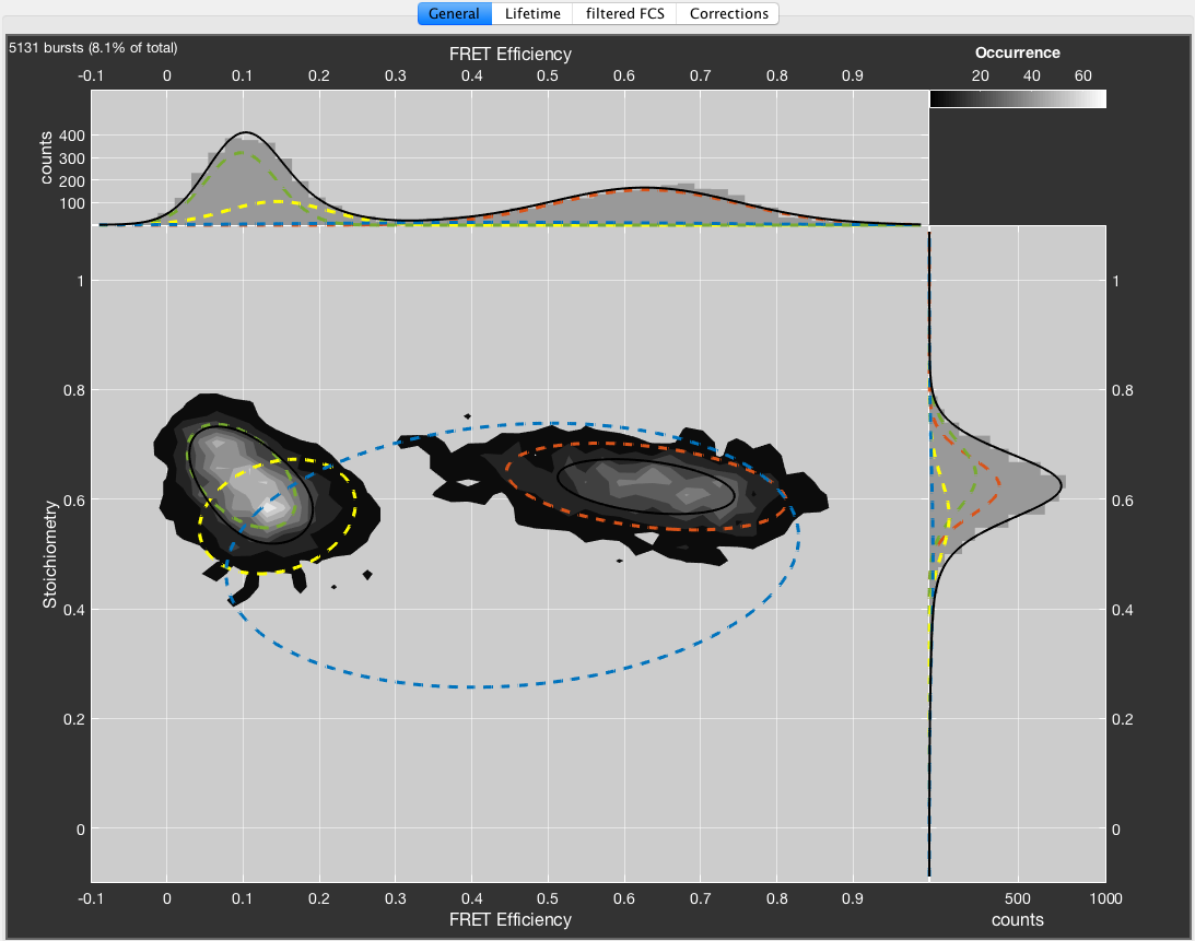
Single-molecule FRET data can be interactively explored using BurstBrowser’s main figure (“General” tab). Parameters are selected using the lists in the “Selection” tab. By default, BurstBrowser plots FRET efficiency vs. Stoichiometry.

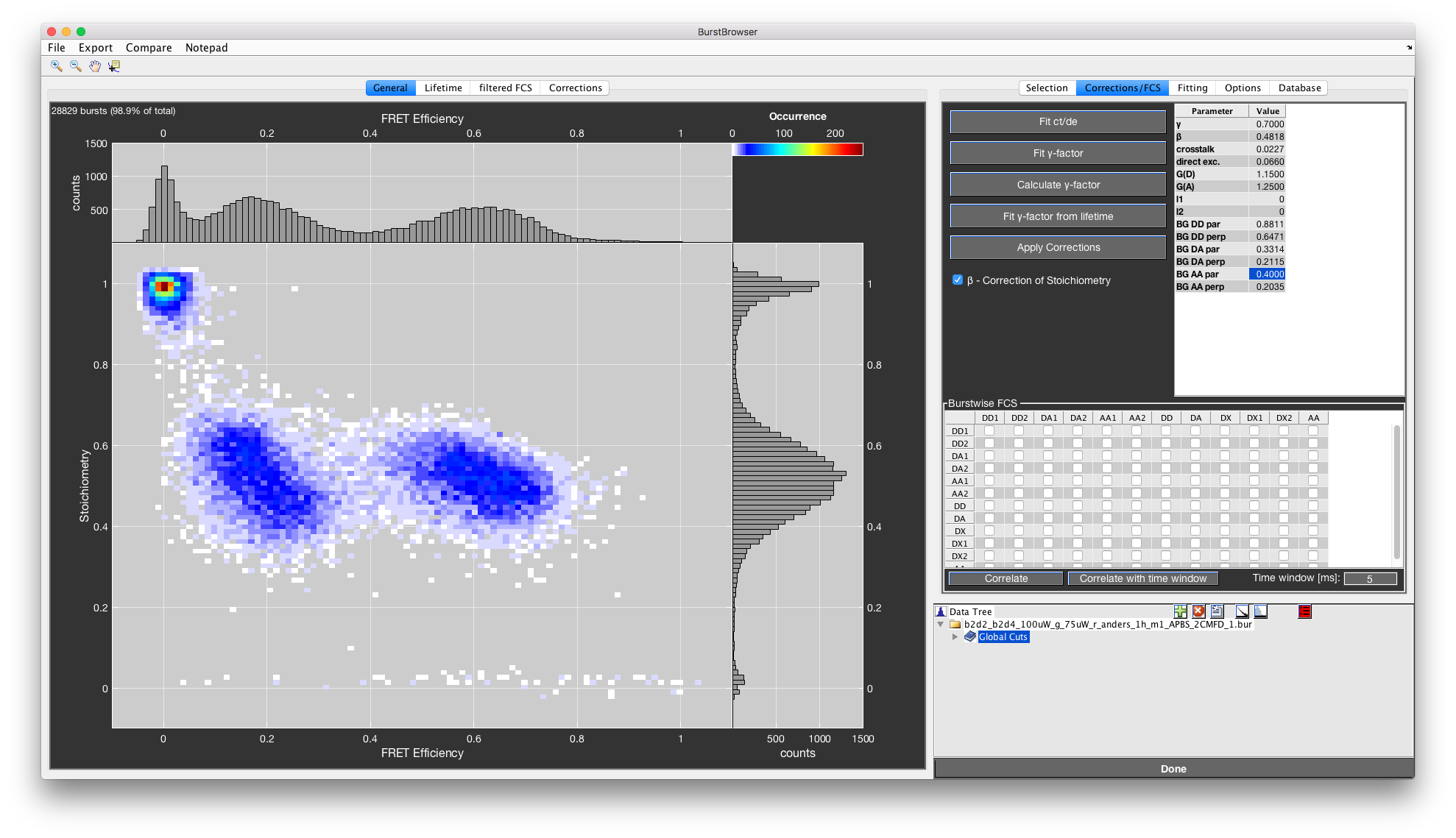
BurstBrowser’s main GUI.

Selecting data

To apply cuts to data, right-click the parameter to add it to the cut table. Here, you can set the lower and upper boundaries for the parameter (“min” and “max”). To temporarily disable the cut, uncheck the “active” checkbox. To remove it completely, click the “delete” checkbox. You can add any combination of parameters.

Using species

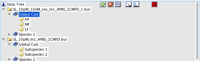
The Species List

Oftentimes, it is helpful to sort the data into different populations or species, which are to be compared with respect to some parameters. BurstBrowser offers a convenient way to do so based on a species/subspecies hierarchy. Species are accessed using the “Data Tree” panel.

By default, BurstBrowser creates a single species called “Global Cuts”, with two subspecies (“Subspecies 1/2”), in addition to the top level tree element showing the filename. You can add species or subspecies by right-clicking an existing species and selecting “Add Species”, which will add an additional species on the same level. Species are removed by clicking “Remove Species”, and renamed by the menu item “Rename Species”.

The general idea of species is to first apply cuts to the measurement to filter out unwanted molecules (i.e. donor- and acceptor-only molecules, photobleaching events, multimolecule events), and subsequently refine the selection in terms of species (i.e. low FRET efficiency, high anisotropy, etc.).

The following rules apply:

• A newly generated subspecies inherits from the parent species.
• Cuts applied to a parent species will automatically be applied to all subspecies, meaning:
  • New parameters will be added to the subspecies.
  • Boundary changes will overwrite boundaries in the subspecies.
• Deleting a parameter from a parent species will remove it from all subspecies.
• Deleting a parameter in a subspecies has no effect on the parent
• Cut boundaries in subspecies can not exceed the boundaries of the parent species.
• The active property is inherited also.

Most functions that can be applied to burst selections can be accessed by right-clicking the species list. Additionally, the species list contains a few buttons in the top right for quick access. These are, from left to right, shortcuts for adding a species, removing a species, renaming a species, exporting the selected species to TauFit, exporting the selected species to PDAFit, and enabling the multiselection mode to compare data sets (see multiselection).

Manual Cut

Manual Cut is available using the crop symbol or by pressing ctrl+space when the main plot is selected. This will turn the cursor into a crosshair that you can use to drag a rectangular selection on the current plot. The defined boundaries will then be applied to the current selected species.

Arbitrary Region Cut (AR)

Arbitrary Region Cut is available by clicking the free selection button or pressing space. Draw a shape in the main plot encircling the population you want to select and confirm the selection by double-clicking the plot. If instead you want to exclude a species from the selection, right-click the Arbitrary Region Cut button and select Invert Arbitrary Region Cut.

Arbitrary Region Cuts can not be modified after they have been defined. In the Cut Table, they will be abbreviated by AR: *, followed by the parameter pair they have been defined on. The *min and max fields have no effect for AR cuts. Like all cuts, if applied to a parent species, they will be automatically applied to the respective child species.

Storing cuts

If you have a set of cuts that you routinely apply to your data (i.e. to select donor-only molecules, or to remove bleaching artifacts…), you can store the cut state and apply it to newly loaded data. Right-click the Cut Table, select Store in cut database and specify a name for the cut state (e.g Donly). Keep the name simple since it will be converted into a valid MATLAB variable name, i.e. all spaces and special symbols will be removed.

After you have defined the cut, it will be shown in cut database popupmenu. To make use of the defined cut state, you can either apply it to the current species using the paint bucket, which will overwrite any existing cuts on the same parameters in the currently selected species, or add a new species with the stored cuts using the plus symbol.

To remove a cut state from the database, right-click the popupmenu and select Remove Cut from Database. To show which cuts a certain stored cut state has defined, click Displayed Selected Cut from Database in the right-click menu. This will show a window with the cut information, and print it to the command line as well.

Note

Arbitrary Region Cuts are not stored in the cut database and simply ignored when saving a cut state.

Synchronizing cuts

When performing a measurement series, you may want to apply the same cuts to a number of files. When multiple files are loaded, you can synchronize cut states between the files by right-clicking the Cut Table and selection Apply current cuts to all loaded files. The cuts of the currently selected species will be applied to all other loaded files. If the file contains a species by the same name, the respective cuts will be overwritten/extended. If the file does not contain a species of the same name, a new species will be created for this file.

Customizing plots

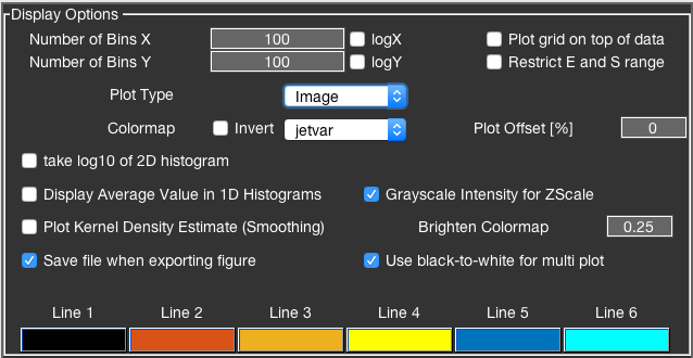
The panel for selecting display options.

BurstBrowser’s plotting functionality and data representation can be modified in a multitude of ways.

Bin numbers for the two-dimensional histograms can be changed independently for x and y dimensions. These settings globally affect the histograms in the “General” and “Lifetime” tabs. Additionally, the logarithm of the x- or y-parameter can be displayed by checking the logX or logY checkboxes.

The plot type for two-dimensional histograms can be chosen between Image, Contour, Scatter and Hex. See the section below section for more details on the plot types.

The colormap can be chosen from a range of standard MATLAB colormaps (jet, hot, bone, gray, parula, etc). Additionally, a variant of the jet colormap is available (jetvar), which starts from white before going through jet’s color palette. All colormaps can be inverted by clicking the checkbox.

To plot the grid lines on top of the data, check the Plot grid on top data checkbox.

To make minor populations more visible, plotting of the logarithm of the frequency information of the two-dimensional histograms is supported. This option only applies to two-dimensional data, while not affecting the one-dimensional histograms.

By checking Display Average Value in 1D Histograms the average value and standard deviation of the respective parameter will be shown in the plots of the parameter histograms.

Enable Save file when exporting figure to automatically trigger a save dialog when closing an export figure.

The Line options allow to set custom colors for lines (i.e. static/dynamic FRET lines, Perrin plots, Gaussian fits). Click the colored box and select a color from dialog to change the line colors.

The other options are specific to other functions of BurstBrowser and are explained in the respective sessions.

Plot types

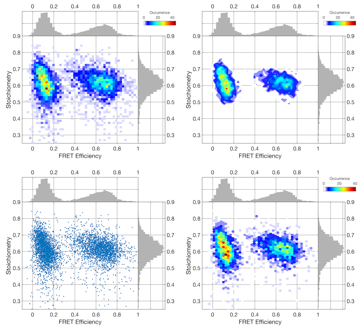
The different plot types supported in BurstBrowser. From top left to bottom right: image, contour, scatter, and hex plot.

Image:

Standard image plot. Can be used with color by parameter. The Plot Offset [%] parameter allows to hide all bins below the given percentage of the maximum value.

Contour:

Contour plot that interpolates the binned data. Can further be customized by specifying the number of contour levels and the contour offset. Contour offset ignores all data below the given threshold, producing cleaner plots, but potentially hiding minor populations. For initial data analysis, it is thus recommended to use image plot, or to set the contour offset to zero. Contour lines can be disabled by unchecking the Plot Contour Lines checkbox.

Scatter:

Scatter plot showing each data point. Can be customized by specifying the marker color and marker size. Can be used with color by parameter.

Hex:

This plot uses hexagonal binning to represent the two-dimensional parameter distribution. Hexagonal binning is a more fitting pattern for round population and can thus represent the distribution better. The plotting is based on hexscatter.m freely available at the MATLAB file exchange.

Kernel density estimation (Smoothing)

Instead of the raw data one can plot smoothed data based on Gaussian kernel density estimation by checking Plot Kernel Density Estimate (Smoothing). This can make it easier to detect populations if low amount of data is available. For kernel density estimation, an important parameter is the width of the Gaussian kernels. We apply the method described in [Botev2010] to determine an appropriate kernel bandwidth automatically from the data, using the script freely available at the MATLAB File Exchange. Kernel density estimation only works with Image and Contour plots. For Scatter and Hex plots the smoothing is only applied to the one-dimensional histograms.

Example of kernel density estimation (left: raw data, right: kernel density estimate)

Color plot by third parameter

Sometimes it can be helpful to investigate three parameters simultaneously. You can color-code a third parameter in the two-dimensional plot using the last column in the cut parameter table (colorbar icon).

Using a third parameter to color-code the E-S plot using the donor anisotropy. From left to right: normal intensity scaling, color-coded without and with intensity scaling, and using the scatter plot. The high FRET efficiency shows higher values for the donor anisotropy due to the shorter donor lifetime.

Color-coding is supported for Image and Scatter plots. The scaling is adjusted to the cut limits of the color-coding parameter. Use the parameter histogram in the top right to adjust the limits. When using an image plot, the parameter histogram for the color-coding parameter in the top right will show the distribution of the pixel-wise average, and thus be different from the burst-wise histogram of the same parameter. For scatter plots, the true burst-wise distribution is shown, since no averaging is needed for color-coding. Thus, when using the image plot, it is advised to set the color-coding parameter cut state to inactive to avoid removing data points when adjusting the cut limits.

You can combine color-coding and intensity information by checking the Intensity scaling for color coding checkbox. Additionally, you can brighten the intensity scaling using the Brighten Colormap option. Color-coding is not compatible with multiselection.

Correcting data

To obtain accurate FRET efficiencies, a number of correction factors is required. Crosstalk, direct excitation and \(\gamma\)-factor can be determined from the measurement directly if PIE is used.

The correction factors are all entered into the Corrections Table found in the Corrections/FCS tab.

The corrections panel.

On first load, the last used corrections are automatically filled into the corrections table. Background count rates are those determined from the specified scatter measurement. If you want corrections to automatically be applied upon load, check the Automatically apply default/stored corrections when loading a file checkbox under Options->Data Processing Options.

Changing parameters

Any parameter can be edited in the Corrections Table, but the changes will only be applied after the Apply Corrections button has been clicked. The Apply Corrections button will turn red to indicate that changes have been performed but not confirmed yet.

The \(\beta\)-factor accounts for different excitation efficiencies of donor and acceptor fluorophore, which cause the stoichiometry value of double labeled molecules to deviate from the theoretical value of \(0.5\). For a correctly chosen \(\beta\)-factor, the stoichiometry is exactly \(0.5\) for a double-labeled species. The correction of the stoichiometry value by the \(\beta\)-factor can be toggled using the respective checkbox.

Note

Correction of the stoichiometry by usage of the \(\beta\)-factor is advised if different interaction stoichiometries are investigated. \(\beta\)-corrected stoichiometries allow to infer interaction stoichiometries directly, i.e. \(S=0.5\) corresponds to a 1:1 stoichiometry, while \(S=0.25\) or \(S=0.75\) correspond to a stoichiometry of 1:3 or 3:1 of donor to acceptor fluorophores, respectively.

Determination of correction factors

Crosstalk and Direct Excitation

To automatically determine the crosstalk and direct excitation correction factors from donor- and acceptor only populations, click the Fit ct/de button. Donor- and acceptor-only populations will be selected based on the stoichiometry (raw) thresholds specified under Options->Data Processing Options. To isolate the acceptor only population, additionally a minimum threshold for the proximity ratio (i.e. the uncorrected FRET efficiency) can be set. To determine proper values for the thresholds, inspect of Stoichiometry (raw) vs. Proximity Ratio.

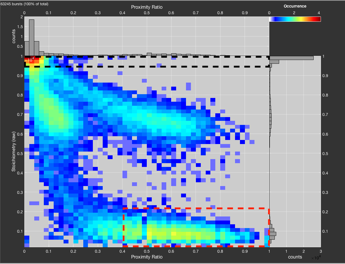
Logarithmic plot of raw stoichiometry vs. proximity ratio to choose thresholds for donor-only (black) and acceptor-only (red) populations. Donor-only is selected by requiring S > 0.95. Acceptor-only is selected by S < 0.22 and proximity ratio > 0.4. Without the proximity ratio the acceptor-only population would be contaminated by molecules from the bridge between acceptor only and low FRET efficiency population.

Histograms of the proximity ratio of the donor-only population and the raw stoichiometry of the acceptor-only populations will be fit with a single Gaussian function to determine the center value. The result is plotted in the Corrections tab, which is automatically given priority. If a single Gaussian is not sufficient to fit the data (adjusted \(R^2<0.9\)), two Gaussian functions are used to fit the data and the center value of the main contribution is used.

Crosstalk and direct excitation are determined from the obtained values \(E_{PR}^{D-only}\) and \(S_{raw}^{A-only}\) by:

\[ \begin{align}\begin{aligned}ct = \frac{E_{PR}^{D-only}}{1-E_{PR}^{D-only}}\\de = \frac{S_{raw}^{A-only}}{1-S_{raw}^{A-only}}\end{aligned}\end{align} \]

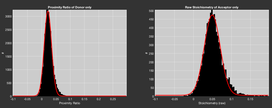
Example for the determination of crosstalk and direct excitation correction factors.

When the parameters for crosstalk or direct excitation are changed following automatic determination, the fits in the plots in the Corrections tab will be adjusted accordingly. Use this to judge if your chosen values are in agreement with the data (i.e. if values have been determined from separate dye measurements).

\(\gamma\)-factor

The \(\gamma\)-factor corrects for different detection efficiencies and quantum yields of donor and acceptor fluorophore. It can be determined from the data in two ways, either using the dependency of FRET efficiency and stoichiometry, or by using the fluorescence lifetime information of the donor fluorophore.

The corrected stoichiometry value should be independent of the observed FRET efficiency, i.e. if the \(\gamma\)-factor is chosen correctly, it the stoichiometry is unaffected by the distribution of the fluorescence signal on the two detection channels. This fact can be used to determine the \(\gamma\)-factor from a measurement of multiple FRET species. For \(\gamma=1\), a linear relation is obtained between the inverse of the stoichiometry and the FRET efficiency [Lee2005]. The fit parameters of the linear fit \(\frac{1}{S} = \Omega+\Sigma \cdot E\) are related to the \(\gamma\)-factor and the \(\beta\)-factor (accounting for different excitation efficiencies, see correction factors):

\[\gamma = \frac{\Omega-1}{\Omega+\Sigma-1}\]

\[\beta = \Omega+\Sigma-1\]

The determination of the \(\gamma\)-factor by this method is implemented in two ways. Fit \(\gamma\) factor uses a burst-wise plot of \(1/S\) vs. \(E\) for \(\gamma=1\) to perform a linear fit using the fit function of MATLAB. To reduce the effect of extreme outliers that occur at small stoichiometry values when taking the inverse, robust fitting by the least absolute residual (LAR) method is applied. The fit result is shown in the bottom left plot in the Corrections tab.

Alternatively, the \(\gamma\)-factor can be calculated directly without fitting if the center points of two different FRET species in the E-S plot are determined. Right-click the Fit \(\gamma\) factor button and select Determine \(\gamma\) factor manually to turn the mouse cursor into a crosshair that you can use to select the centers of two different FRET species sequentially in the E-S plot shown in the bottom left plot of the Corrections tab.

The most robust way to determine the \(\gamma\)-factor is to determine the E-S values for \(\gamma = 1\) for different populations using the Gaussian fitting module. Once determined, you can calculate the \(\gamma\)-factor by clicking the Calculate \(\gamma\) factor button and inputting the values into the table. Optionally, one can specify the uncertainty for E and S (\(\sigma E\) and \(\sigma S\)), which will be used to estimate the error in the determined \(\gamma\)- and \(\beta\)-factors. Note that the uncertainty in E and S is not given by the standard deviation as obtained from the fit. A more appropriate estimate for the uncertainty would be the standard error of the mean given by \(SEM = \sigma/\sqrt{N}\), where \(N\) is the number of data points, i.e. bursts, used for the fit.

If the fluorescence lifetime information of the donor is available, you can determine \(\gamma\) even if only a single FRET population is available, as long as the measured system is static, i.e. shows no FRET dynamics (e.g. a DNA molecule). Clicking Fit \(\gamma\) factor from lifetime will minimize the deviation of the FRET species from the theoretical static FRET line defined by the donor-only lifetime, the Förster radius and the observed linker length. The fit routine uses robust fitting by the bisquare method. The result is displayed in the bottom left plot of the Corrections tab. For more information on the dependence between the FRET efficiency and the fluorescence lifetime of the donor, see the respective section on the static FRET line.

Note

The \(\gamma\)-factor can also be determined by inspecting the E-\(\tau_D\) plot and manually varying \(\gamma\) until the population falls onto the static FRET line. This is advised if the automatic fitting does not yield satisfying results.

In all cases, the currently selected bursts are used for the automatic determination. Ensure that only double labeled molecules are selected. If no single measurement with multiple FRET species is available, you can combine separate measurements of different FRET species using the multiplot functionality to plot them simultaneously. The automatic determination will use the currently selected bursts, and combine the selection over multiple files.

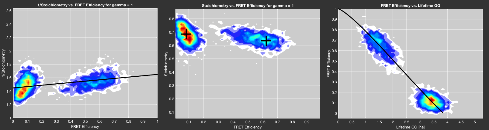
Determining the \(\gamma\)-factor. (Left) Fit of 1/S vs. E. (Middle) Manual selection of the center points of the population. (Right) Using the fluorescence lifetime of the donor fluorophore.

Synchronizing correction factors

To synchronize correction factors between all loaded files, right-click the Apply Corrections button and select Replace corrections of all files with current one. This will overwrite the correction parameters of all other files with the current one.

Comparing datasets

Multiselection

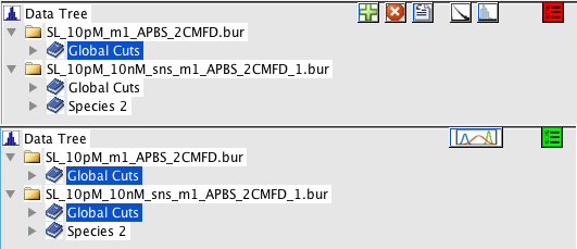
The MultiSelection button in the top right of the Species List toggles the multiselection mode. Top: multiselection disabled, bottom: multiselection enabled. Enabling the multiselection mode display the MultiPlot button, while hiding the buttons associated with single species.

Multiselection mode is activated by clicking the MultiSelection button in the Species List (see Species List), which will allow multiple species in the Species List to be selected simultaneously. The button turns red when MultiSelection is disabled, and green when it is enabled. This will disable all options associated with the Species List that are related to single files. Multiselection works between different files.

Selecting multiple species simultaneously will superimpose all selected datasets. Multiselection works with all functions to determine correction factors. While the two-dimensional plot will only show the superposition of all selected species, the marginal distributions will show histograms for the individual species. When using the Scatter plot, species will additionally be color-coded in the two-dimensional plot.

By default, the selected species are area-normalized. This is ensures that all species are visible, even if there are large differences in the number of bursts per species. The histograms can alternatively be normalized to their maximum value by right-clicking the MultiSelection button and selecting Normalize to… -> maximum. You can disable the normalization by right-clicking the Multiselection checkbox and unchecking Normalize populations. The display of the sum of all selected populations can be toggled in the same right-click menu by deselecting the Display sum of all populations option.

Multiselection using Image plot will superimpose the populations in the two-dimensional plot, but show the individual populations in the marginal distributions. The Scatter plot shows the different populations using different colors. The Multiplot functionality color-coded the populations.

The Multiplot button allows for up to three species to be plotted simultaneously using a separate color for each species (blue, red and green in that order). It appears in the top right of the Species List when the MultiSelection mode is activated. If more than three species are selected, the first three will be used. Two coloring modes are available that can be changed under Options->Display Options. The default mode uses RGB channels to display the different species. Occurrence is encoded by color intensity for every color channel, starting from white. High intensity regions of overlapping species will be black in this mode. Alternatively to RGB, a “black-to-white” mode is implemented, which starts at black color for low intensity going to white at high intensity.

Multiplot of two species using white-to-black mode (left) and black-to-white mode (right).

Hint

If more than three species need to be visualized simultaneously, it is best to use a Scatter plot together with multiselection.

Comparing single parameters

The most common case when analyzing multiple data sets is to compare the FRET efficiency histograms of separate measurements. This is available by clicking through the Compare menu in the toolbar. Select Compare FRET histograms of loaded files to create a single plot with all FRET efficiency histograms, using the last selected species of the respective files. If another parameter is to be compared, select Compare current parameter of loaded files instead. This will use the currently selected parameter for the x-axis, i.e. in the left parameter selection list.

To compare parameters of different species from the same measurement (or between measurements), enable the Multiselect checkbox and select the species to be compared. Compare -> Compare current parameter of selected species will again use the currently selected x-axis parameter.

When comparing FRET efficiency histograms, e.g. from a time series, one can also display a waterfall plot by enabling the Make waterfall plot when comparing FRET histograms in the Options -> Data processing tab.

Using the lifetime information

The fluorescence lifetime information is an important parameter in burst analysis. It allows to identify photophysical artifacts like quenching, and, together with the anisotropy information, the rotational freedom of the fluorophore can be addressed. Furthermore, it serves as a parameter to identify conformational dynamics on the burst timescale. BurstBrowser gives an overview over the most important lifetime-related plots in PIE-MFD in the Lifetime tab. These plots should be carefully inspected for all PIE-MFD measurements.

The Lifetime tab showing all important lifetime-related plots.

The settings for fits in the Lifetime tab, found under the Fitting tab.

In addition to the overview given in the Lifetime -> All tab, the Individual tab allows to inspect the lifetime-related plots individually using a larger plot with additional marginal distributions. Use the list in the top right to change the current plot. All fits can also be performed in the Individual plot.

E vs. \(\tau_{D(A)}\)

The top-left plot shows the FRET efficiency plotted versus the fluorescence lifetime of the donor (in presence of the acceptor, \(\tau_{D(A)}\)). In theory, the dependence between FRET efficiency is linear and given by the so called “static FRET line”:

\[E = 1-\frac{\tau_{D(A)}}{\tau_{D,0}}\]

where \(\tau_{D,0}\) is the lifetime of the donor in the absence of the acceptor. Practically, the plot deviates from the theoretical line because the dyes are attached to linkers, leading to fast fluctuations (~100 ns) in the donor-acceptor distance even for static samples that are averaged on the burst timescale (~ms). Since the lifetime fit is performed only on the donor fluorescence decay, low FRET efficiency states contribute more photons to the decay, and the determined lifetime is thus biased towards long lifetimes. This effect leads to a slight curving of the theoretical static FRET line, which depends on the Förster radius and the apparent length of the linker, i.e. the magnitude of the distance fluctuations. The apparent linker length can be determined from a TCSPC analysis of a static FRET sample by fitting a distance distribution, and is usually on the order of 5-6 Angstrom.

Equivalently, conformational dynamics during bursts will lead to mixture of states. While the FRET efficiency is averaged based on the time the molecule spent in the states, the fluorescence lifetime is again biased by the brightness of the species and thus biased towards the low FRET efficiency, long fluorescence lifetime state. In the absence of linker dynamics, the dynamic FRET lines between two states (1 and 2) with different FRET efficiencies is given by:

\[E = 1-\frac{\tau_1\tau_2}{\tau_{D,0}\left(\tau_1+\tau_2-\left<\tau\right>_f\right)}\]

Here, \(\left<\tau\right>_f\) is the intensity-weighted lifetime as determined by the burst-wise fit. Note that there is no analytical expression for static or dynamic FRET lines when linker dynamics are to be considered.

To correctly account for the linker dynamics, the static and dynamic FRET lines in BurstBrowser are simulated as described in the supplementary information to [Kalinin2010], taking the linker dynamics into account. However, in contrast to what is described in [Kalinin2010], no approximation by a third-order polynomial is performed in BurstBrowser; instead, the calculated lines are used directly without the intermediate step of approximation because the simulation is fast.

Plotting the static FRET line

The static FRET line is a function of the donor-only lifetime, the Förster radius and the apparent linker length. It can be plotted by clicking the Plot static FRET line button and is updated when any of the related parameters are modified.

Using the dynamic FRET line

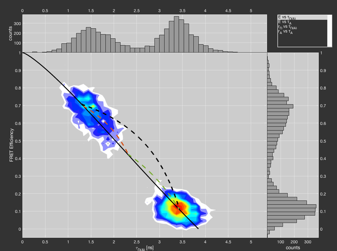
An example of static and dynamic FRET lines. Dynamic FRET lines are plotted between the two states (black) and additionally for a hypothetical intermediate state (red and green).

Click the Dynamic FRET line to define a dynamic FRET line. This will turn the cursor into a crosshair, allowing you to define the two states belonging to the dynamic FRET line by clicking into the respective plot. You can plot up to three dynamic FRET lines together. Add more dynamic FRET lines by right-clicking the plot instead of left-clicking.

Alternatively, you can right-click the button and select Define States to manually define the two states by their respective lifetime. Choose which line you want to define, up to three lines maximum. Remove individual lines by right-click the Dynamic FRET line button and selecting Remove Plot to specify the number of the line you want to remove. Line colors correspond to the settings in the Options tab. Dynamic FRET lines will not updated if related parameters are changed.

Hint

Use sub-ensemble TCSPC and a biexponential lifetime fit to determine the fluorescence lifetimes of the two states if the dynamics are fast.

Getting donor-only and acceptor-only lifetimes

Donor- and acceptor-only lifetimes can be extracted from the donor- and acceptor-only subpopulations of the experiment. This gives an intrinsic reference for the static FRET line and removes the necessity to determine the donor-only lifetime from a reference sample.

The donor- and acceptor-only lifetimes can be determined in two principal ways: from the burst-wise lifetime distributions, or from a sub-ensemble TCSPC analysis.

The former is automated in BurstBrowser. Simply click the Get dye lifetimes from data button in the Fitting tab (subsection Lifetime Plots). This will automatically select donor- and acceptor-only populations and determine the mean burst-wise lifetime by Gaussian fitting. The fit can be inspected in the Corrections tab in the top two plots (the same plots previously used for inspecting the quality of the crosstalk and direct excitation fits). The values for donor- and acceptor-only lifetimes will be automatically updated.

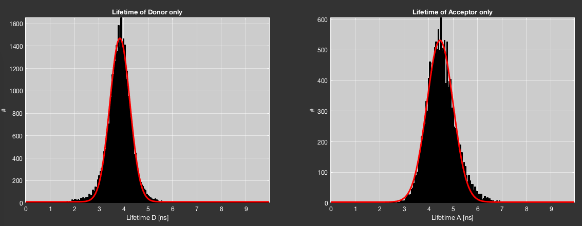
Example fits of donor- and acceptor-only lifetime distributions.

Sub-ensemble TCSPC analysis can be manually performed on selected donor- and acceptor-only populations as described in the corresponding section. Determined lifetimes can be manually input into the edit boxes.

Anisotropy vs lifetime

The measured steady-state anisotropy depends on the fluorescence lifetime. Since the anisotropy itself decays, a shorter fluorescence lifetime will result in a higher averaged anisotropy than a long fluorescent lifetime at equal rotational correlation time. The dependance between anisotropy and lifetime is given by the Perrin equation, assuming single exponential lifetime and anisotropy decays:

\[r\left(\tau\right) = \frac{r_0}{1+\frac{\tau}{\rho}}\]

Here, \(r_0\) is the fundamental anisotropy of the fluorophore and \(\rho\) is the rotational correlation time.

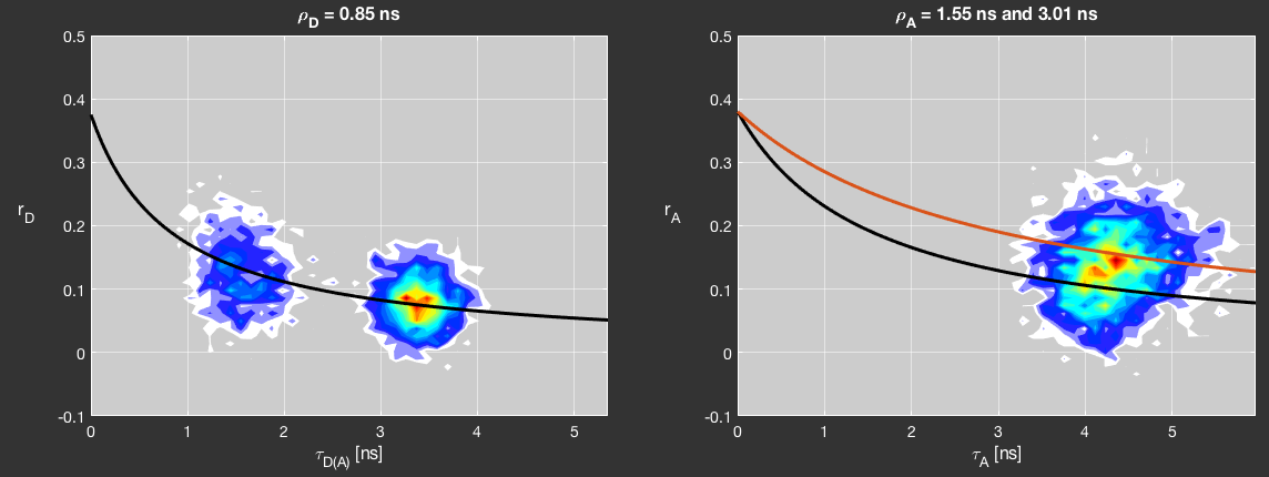
An example of Perrin plots.

You can add Perrin lines to the anisotropy plots to distinguish species based on their rotational correlation time. Clicking the Fit Anisotropy button to fit Perrin lines to the \(r-\tau\) distribution. Determined rotational correlation times will be shown above the plots. You can manually add Perrin lines by clicking the Manual Perrin line button and selecting a population in the plot. Add up to two more Perrin lines by repeating the previous step but right-clicking the plot. Perrin lines will use the specified \(r_0\) values for the respective colors. Reset any present Perrin fits by either clicking the Fit Anisotropy button or defining a new primary Perrin line using the Manual Perrin line button.

Lifetime/anisotropy fitting by sub-ensemble TCSPC

You can perform sub-ensemble (or burst-selective) TCSPC analysis on a species by selecting it in the species list in the bottom right of the Selection tab, right-clicking and selecting Send selected species to TauFit. Alternatively, you can click the small fluorescence decay symbol at the top of the species list. This is only enabled if Multiselect is disabled, since you can only send single species to TauFit. This will open an instance of TauFit with the cumulative data of all selected bursts. You can use the whole toolset of TauFit as described in the TauFit manual.

Instead of selecting PIE channels, you will be able to select FRET channels, i.e. DD, AA, and AD for two-color FRET. TauFit will use the instrument response function and scatter/background pattern that is stored with the burst measurement. The FRET-sensitized acceptor decay (DA) is a convolution of FRET-quenched donor decay and acceptor decay, for which no model is supplied in TauFit. However, the residual anisotropy of donor, acceptor and FRET-sensitized acceptor emission can be used to gain information about the distribution of the orientational factor \(\kappa^2\), as described in the respective section of the TauFit manual.

Fitting data using Gaussian distributions

BurstBrowser allows to fit any combination of parameters in the General plot using a Gaussian mixture model with up to 4 components, using either a maximum likelihood estimator (MLE) or by minimizing the squared error (LSQ). Select the fit method from the bottom dropdown menu and the number of Gaussian distributions to be used from the top dropdown menu (currently, up to 4 species are available). Checking the Pick start points manually checkbox will allow you to manually specify start points for the fit algorithm by clicking in the plot.

The fit model \(M\) is given by a superposition of \(N\) bivariate normal distributions with amplitude \(A\), mean value vector \(\mu\) and covariance matrix \(\Sigma\):

\[M(x,y) = \sum_{i=1}^N A_i\cdot\left(2\pi\right)^{-1}\left|\Sigma_i\right|^{-1/2}\exp\left[-\frac{1}{2}\left(x-\mu_i\right)'\Sigma_i^{-1}\left(x-\mu_i\right)\right]\]

The parameters of the fit model are the fractional contributions of each species, the center points in X and Y dimensions Mean(X) and Mean(Y), as well as the corresponding distributions widths \(\sigma(XX)\) and \(\sigma(YY)\) and covariance between the parameters COV(XY).

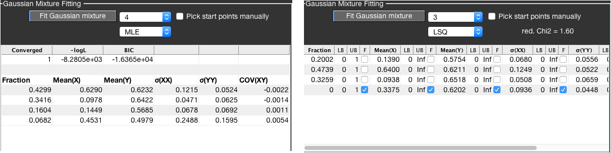
Gaussian mixture fitting user interface for MLE (left) and LSQ (right).

Example result of Gaussian mixture fitting.

Note

The ellipses for the individual populations are isolines of the distributions. You can specify the isoline height using the Isoline height for Gaussian fit display options between 0 and 1. The colors for the populations are given by the Line Colors.

Hint

To easily export the fit result, right-click the table and select Copy fit result to clipboard to transfer the data to a spreadsheet.

MLE fitting

Fitting of Gaussian distributions using maximum likelihood estimation is implemented using the fitgmdist function of MATLAB. The algorithm operates on the raw data and is thus independent of the used binning for the 2D plot. MLE fitting does not allow for fixing of parameters or restriction via lower and upper boundaries. The MLE fit additionally returns information on convergence (0 if the fit did not converge, 1 otherwise), the negative logarithm of the likelihood at the found minimum (-logL) and the Bayesian information criterion (BIC), defined as:

\[BIC = -2\ln\mathcal{L}+\ln(n)k\]

Here, \(\mathcal{L}\) is the likelihood of the model, \(n\) is the number of data points and \(k\) is the number of free fit parameters. Use the BIC to decide how many distributions are needed to describe the data; the model with the lowest value for the BIC should be preferred. See the wikipedia page for more information on the BIC.

LSQ fitting

The least-squares fitting routine minimizes the squared error between data and model using the lsqcurvefit function of MATLAB. You can fix parameters (F)and set their lower and upper boundaries (LB and UB) in the fit parameter table. The LSQ fit will return the reduced chi-squared (red. Chi2, \(\chi^2_{\mathbf{red}}\)) as a measure for the goodness-of-fit, defined by:

\[\chi^2_{\mathbf{red}} = \sum_{x,y} \frac{\left(D(x,y)-M(x,y)\right)^2}{D(x,y)}\]

Here, the \(\chi^2_{\mathbf{red}}\) is calculated assuming Poissonian statistics for estimating the uncertainty in the data. Note that while the \(\chi^2_{\mathbf{red}}\) is reported, the fit routine is solely based on the squared error and not the \(\chi^2_{\mathbf{red}}\).

1D parameter fit

Single parameter fits using the above described methods can be performed by simply selecting the same parameter for x- and y-coordinates.

Fitting of FRET efficiency histograms with customizable model functions is additionally implemented in FCSFit.

Defining species from fit result

The obtained fit result can be used to sort bursts into species. Bursts belonging to a certain bin in the 2D plot will be assigned to the different fit species based on the relative contributions of the fit species. This functionality is accessed by right-clicking the fit result table and selecting Define species from fit. A new selection will be added to the species list, encompassing all selected bursts used for the fit.

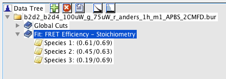
Burst selection defined from fit result. Species 1 was defined from the fitted component with mean values for FRET efficiency = 0.61 and Stoichiometry = 0.69.

The name for the parent species contains the used parameters for the fit. The subspecies names contain the center values of the respective parameters that were used to define the species.

Hint

This functionality can in principle be used to remove “background” species from the analysis. However, assignment of “background” signal needs to be justified by control measurements. If, for example, the used buffer contains fluorescent contaminations, a burst analysis on buffer-only can identify the background.

FCS analysis

Burst-wise FCS

Burst-wise FCS can elucidate differences in diffusion time and thus interactions or conformational dynamics on the sub-millisecond timescale. When calculating correlation functions on time scales similar to the length of the recorded signal, as is the case for burst-wise FCS, sampling artifacts need to be considered. In other words, long time lags e.g. on the timescale of diffusion are sampled less frequently in burst-wise time traces than short time lags. For a given time lag \(\tau\) and burst duration \(T\), the time lag can only be sampled for photons detected in the range \(\left[0,T-\tau\right]\). In practice, individual correlation functions are calculated for every contributing burst and subsequently averaged while taking care of the uneven sampling:

\[G_{\mathbf{bw}}\left(\tau\right) = \frac{\sum_{k} n_k(\Delta t = \tau) \sum_{k} \left(T_k-\tau\right)}{\sum_{k} n_k(t\leq T_k-\tau)\sum_{k} n_k(t\geq\tau)}\]

Here, the sums go over the number of bursts \(k\), \(n_k(\Delta t = \tau)\) is the number of photon pairs in burst \(k\) with time lag \(\tau\), \(T_k\) is the burst duration, and \(n_k(t\leq T_k-\tau)\) and \(n_k(t\geq\tau)\) are the number of photons in the interval \([0,T_k-\tau]\) and \([\tau,0]\).

Burst-wise FCS can detect conformational dynamics on timescales faster than the diffusion. The diffusion time determined by burst-wise FCS, however, is strongly dependant on the chosen burst search parameters, i.e. higher photon count thresholds will terminate the burst earlier, leading to shorter burst durations. This effect can be diminished by adding a time window around the bursts, enabling a more accurate determination of the diffusion part of the FCS curve. Another effect of the burst selection is that regions of high count rate are selected from the measurements for correlation, resulting in reduced fluctuations and thus lower FCS amplitudes since the average intensity is overestimated. Additionally, since correlating regions are selected, the correlation function usually does not diminish to 0 at large time lags, requiring a significant offset to be considered in the model function.

The figure below illustrates the effect of the chosen time window on the shape and amplitude of the obtained burst-wise FCS curves. A larger time window results in higher amplitudes of the correlation function. The burst-wise FCS curve underestimates the diffusion time, which is asymptotically increased with increasing time window. Obviously, also the maximum time lag scales with the chosen time window. Since the time window is added both to the start and end of the bursts, the maximum lag time will be approximately twice the time window size.

See [Laurence2007] for more information on burst-wise FCS.

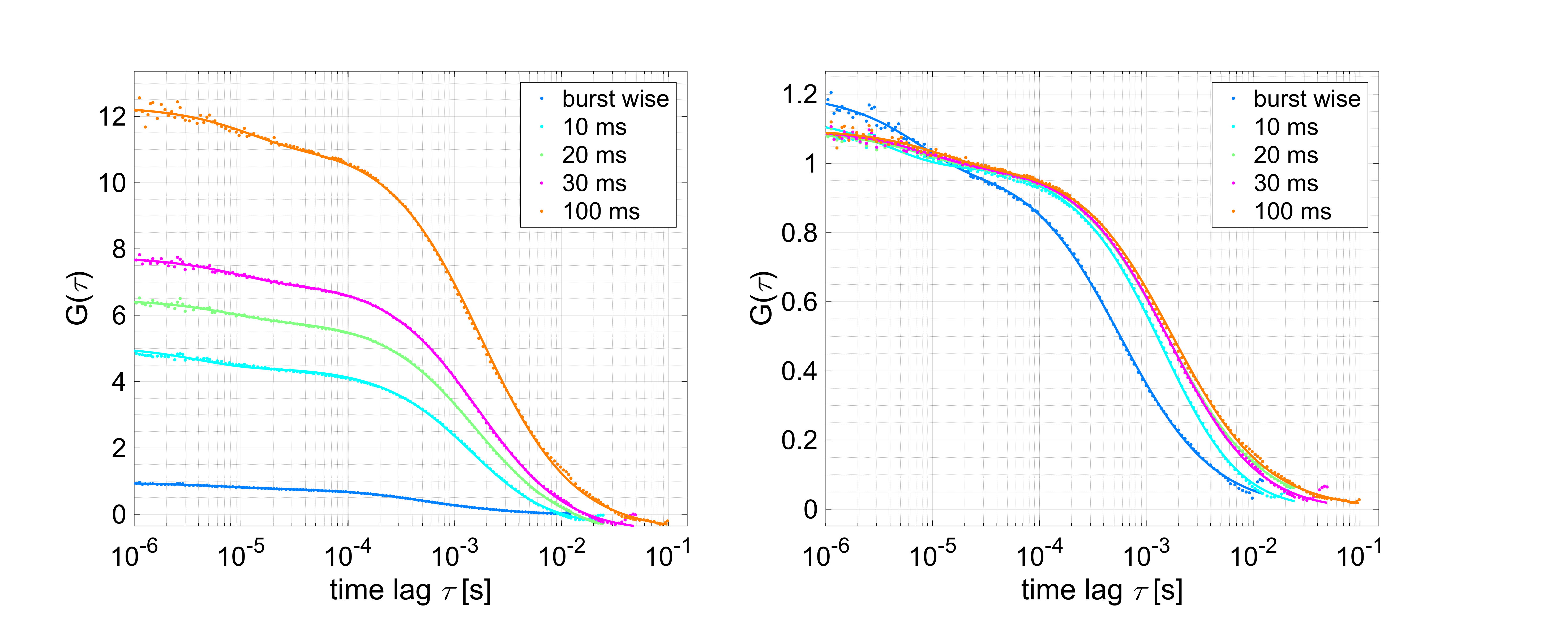
Burst-wise correlation with increasing time window, unnormalized (left) and normalized to the fitted number of particles (right). For all curves the offset has been subtracted.

When adding a time window, it is possible that adjacent single molecule events fall into the region around the respective burst, leading to contamination of the species-selective correlation function. If another single molecule event that was detected by the burst search falls into the time window around a contributing burst, the burst is not included in the correlation function. This will ensure that the obtained correlation function is specific to the selected species. However, contribution of contaminating signal that was not detected as burst will not be filtered out.

Note

Generally, for burst-wise FCS, it is recommended to use low intensity thresholds for the burst search to detect as much of the fluorescence signal of the single molecules as possible, smoothing the edges of the burst-wise correlation function. Additionally, if species-selective FCS analysis is to be performed, the concentration should be chosen sufficiently low to leave enough time between individual events.

Using the burst-wise FCS module

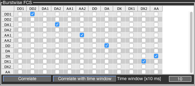
The burst-wise FCS GUI in the Corrections/FCS tab.

To perform burst-wise FCS analysis, BurstBrowser pre-defines combinations of PIE channels, namely the channels DD for donor fluorescence after donor excitation, DA for acceptor fluorescence after donor excitation, AA for acceptor fluorescence after acceptor excitation and DX = DD + DA, i.e. all photons after donor excitation. Parallel and perpendicular polarization channels are indicated by number (1 is parallel, 2 is perpendicular), thus DX1 = DD1 + DA1. When no number is given, the channel combines both polarizations, e.g. DD = DD1 + DD2.

FRET-FCCS analysis requires the autocorrelations and the cross-correlation of the donor and FRET signals, i.e. in terms of PIE channels the correlation functions for DD1 x DD2, DA1 x DA2 and DD x DA. Note that for the autocorrelations, channels with different polarization should be cross-correlated to avoid detector artifacts like dead time or afterpulsing. On the other hand, for the cross-correlation the polarization channels should be combined, i.e. (DD1+DA2) x (DD2+DA2), to ensure that all photon information is used. Other relevant FCS curves for FRET-FCCS analysis are the autocorrelation of the acceptor signal after acceptor excitation AA1 x AA2, as well as the autocorrelation of the total signal after green excitation DX1 x DX2, which will not be sensitive to FRET dynamics.

A default selection of these correlation functions can be set by right-clicking the table and selecting FRET FCCS selection. Likewise, the selection in the table can be reset by clicking Reset. The divider coarse-grains the time resolution of photon arrivals; its function is describe in this section.

Click the Correlate button to perform burst-wise FCS without any time window, and the Correlate with time window button for correlation with time window. The time window is specified in units of 1 ms. The chosen time window will be added before and after the burst, resulting in a total signal trace length of twice the time window. A time window can only be included if the Save total photon stream option was selected for the burst analysis. See the burst search section in the PAM manual for more details.

Burst-wise diffusion time and diffusion coefficients

The burst-wise correlation can also be used to determine a burst-wise diffusion time by fitting of the individual correlation functions for every single molecule event. To use all available signal, the correlation function is computed from all photons belonging to a burst (i.e. GG1+GG2+GR1+GR2+RR1+RR2). Any channel selections in the correlation table are thus disregarded. Since the burst-wise correlation functions are undersampled and thus noisy due to the limited number of photons per burst, a simple 2D diffusion model is used to fit the burst-wise diffusion time \(\tau_D\):

\[G(\tau) = \left(1+\frac{\tau}{\tau_D}\right)^{-1}\]

Correlation functions are fitted in the rang of 10 \(\mu s\) up to one tenth of the signal trace length. The amplitude parameter is eliminated from the fit procedure by normalizing the correlation function to the average of the first 10 data points. Burst-wise fitting of correlation functions only yields useful results when adding a time window around the bursts. When used only on the burst signal trace, diffusion times are underestimated. The diffusion coefficient is calculated by:

\[D = \frac{\omega_r^2}{4\tau_D}\]

To access this functionality, right-click the Correlate with time window button and select Fit burst-wise diffusion time. The functionality is only available with the usage of time windows around the burst

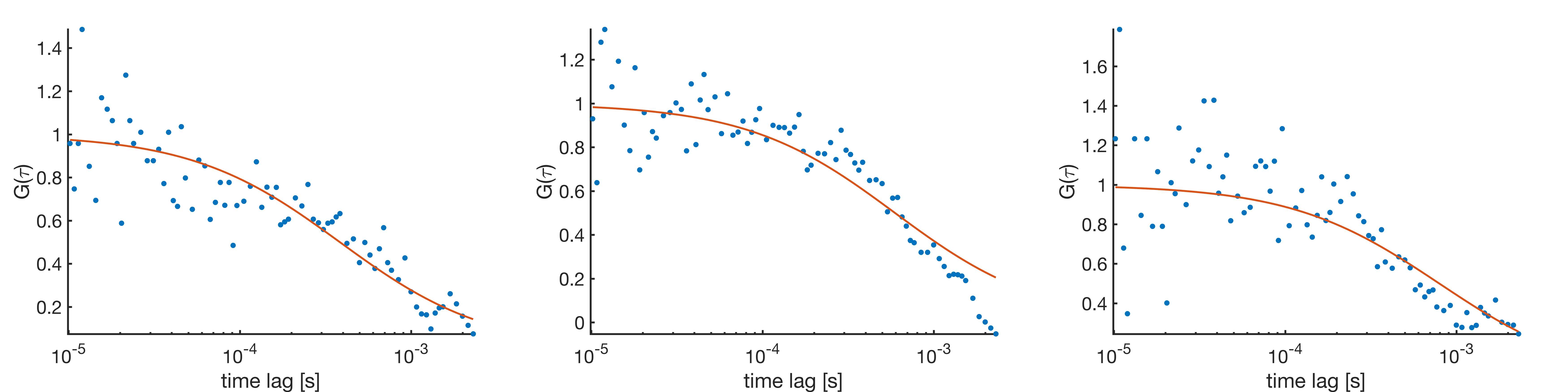
Examples of burst-wise correlation functions and fits. Time window length is 10 ms.

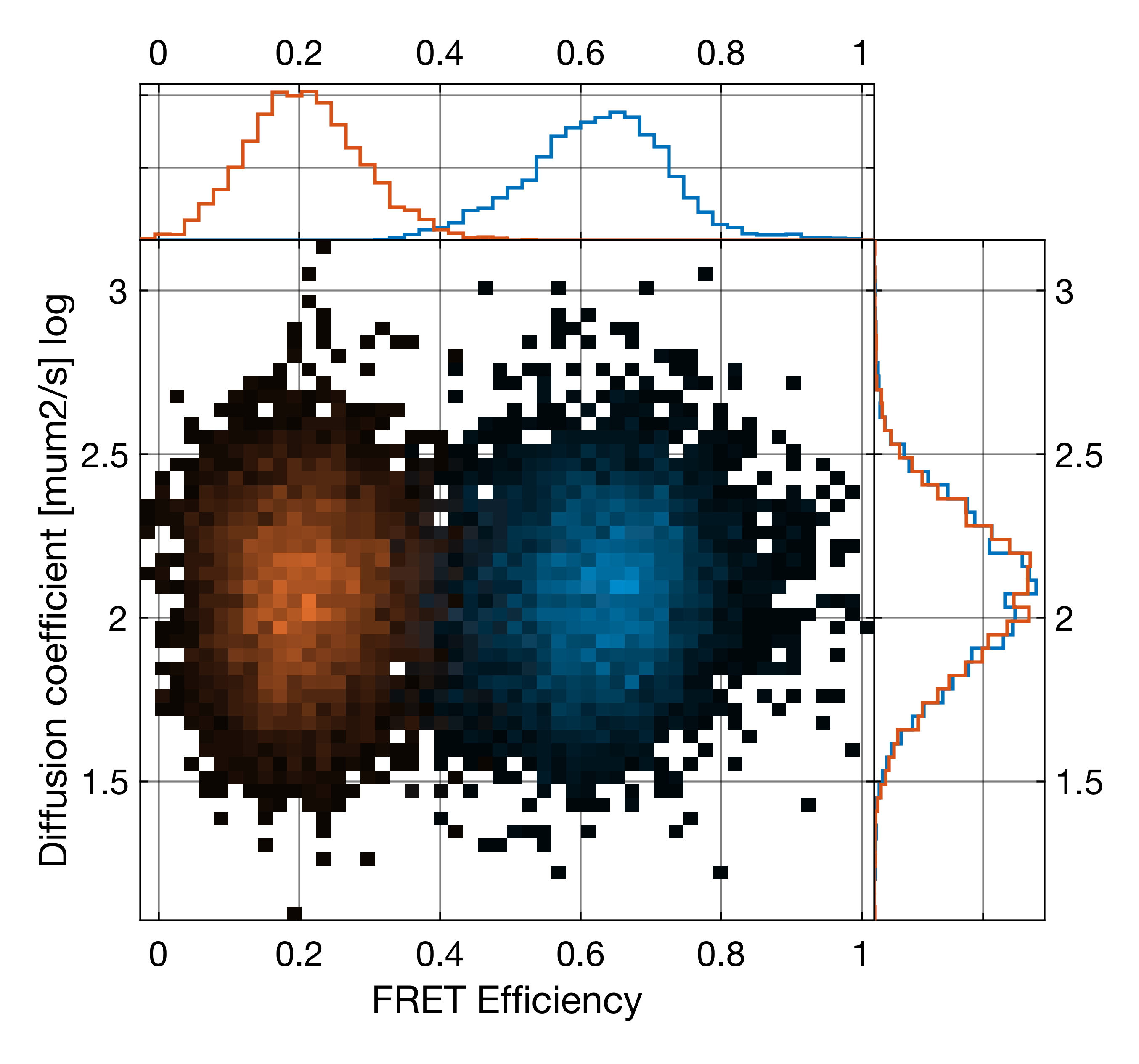
Example of burst-wise diffusion coefficient analysis. Shown is a measurement of two DNA molecules with identical structure, but different labeling position, showing different FRET efficiencies but identical diffusion coefficient distributions (shown is the logarithm of the diffusion coefficient).

Note

Choose a large enough time window (> 5 ms) to ensure that the diffusion coefficient is not overestimated due to the burst-search algorithm.

Using the filtered-FCS module

Filtered FCS is an extension of fluorescence lifetime correlation spectroscopy (FLCS), extending the theory to include other parameters in addition to the fluorescence lifetime that are available in MFD, e.g. the fluorescence anisotropy and color information (i.e. FRET efficiency). See the corresponding section in the PAM manual.

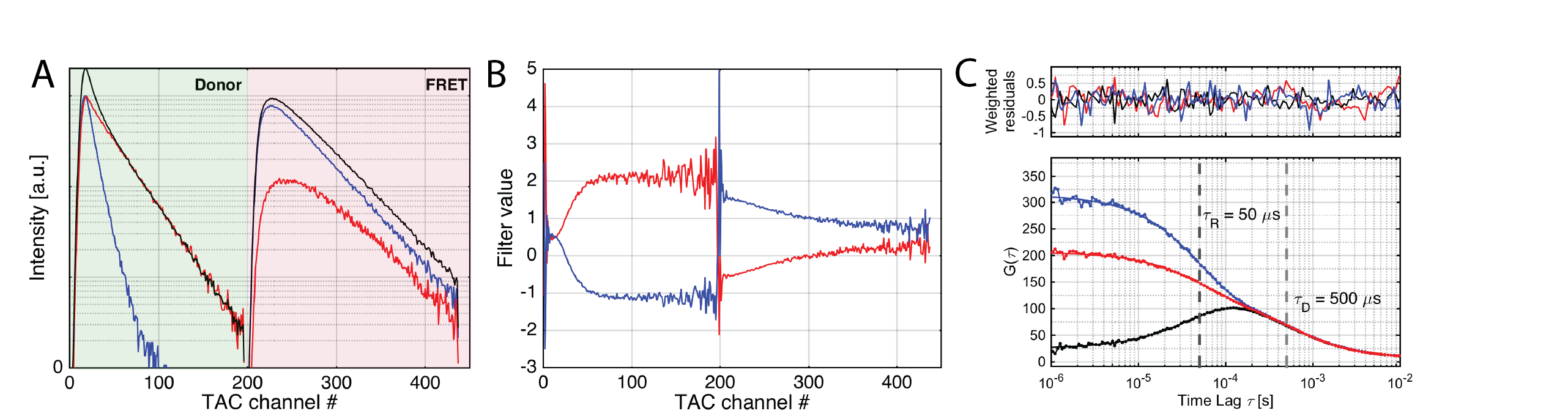
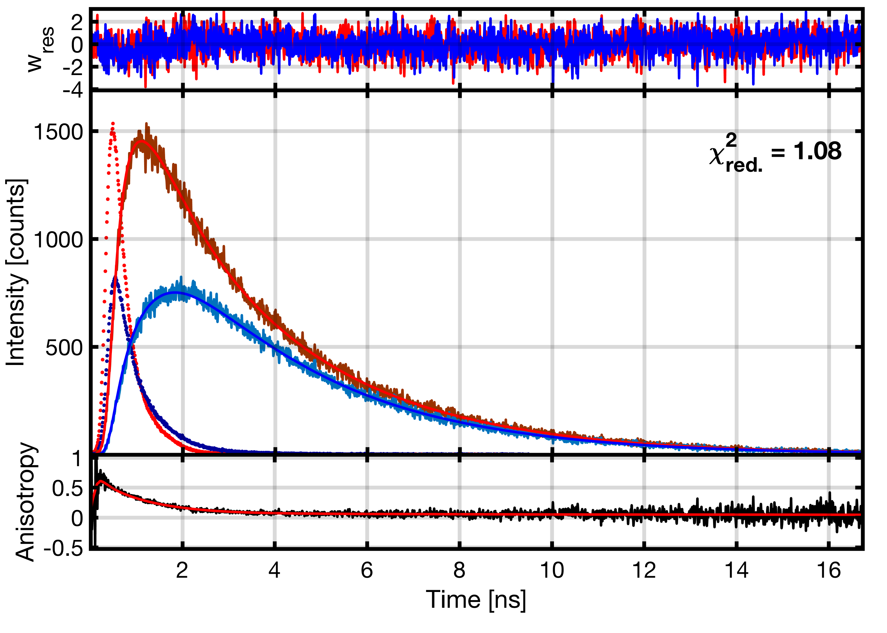
An example of filtered FCS analysis. (A) Stacked microtime histograms of the measurement of the mixture (left) and the high and low FRET efficiency species (blue and red). Donor and FRET-sensitized acceptor microtime histograms are stacked to use the color information in filter generation. (B) Corresponding statistical filters. (C) Resulting species auto- and cross-correlation functions.

To resolve dynamics in the sub-nanosecond range, fFCS requires cross-correlation between two detectors to avoid dead time and other electronic artifacts. fFCS is thus only implemented for setups using two detection channels per color, either split by polarization or using a 50:50 beam splitter. Separate filters are generated on the two independent detection channels, which are cross-correlated when calculating the correlation functions.

Filtered-FCS functionality is integrated into BurstBrowser, allowing the use of subsets of bursts to define the filters for the pure species.

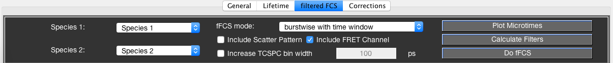
Filtered-FCS options panel

The filtered-FCS module requires the definition of a parent species in the Species List with at least two child species, representing different subsets of the parent species. BurstBrowser will then treat the parent species as the total measurement, which will be described as a superposition of the sub-species.

The functionality of the filtered-FCS module will be demonstrated using the data set shown in the following figure. In the measurement, fast fluctuations between low and high FRET efficiency states are observed on the \(\mu s\) timescale, as indicated by the deviation from the static FRET line.

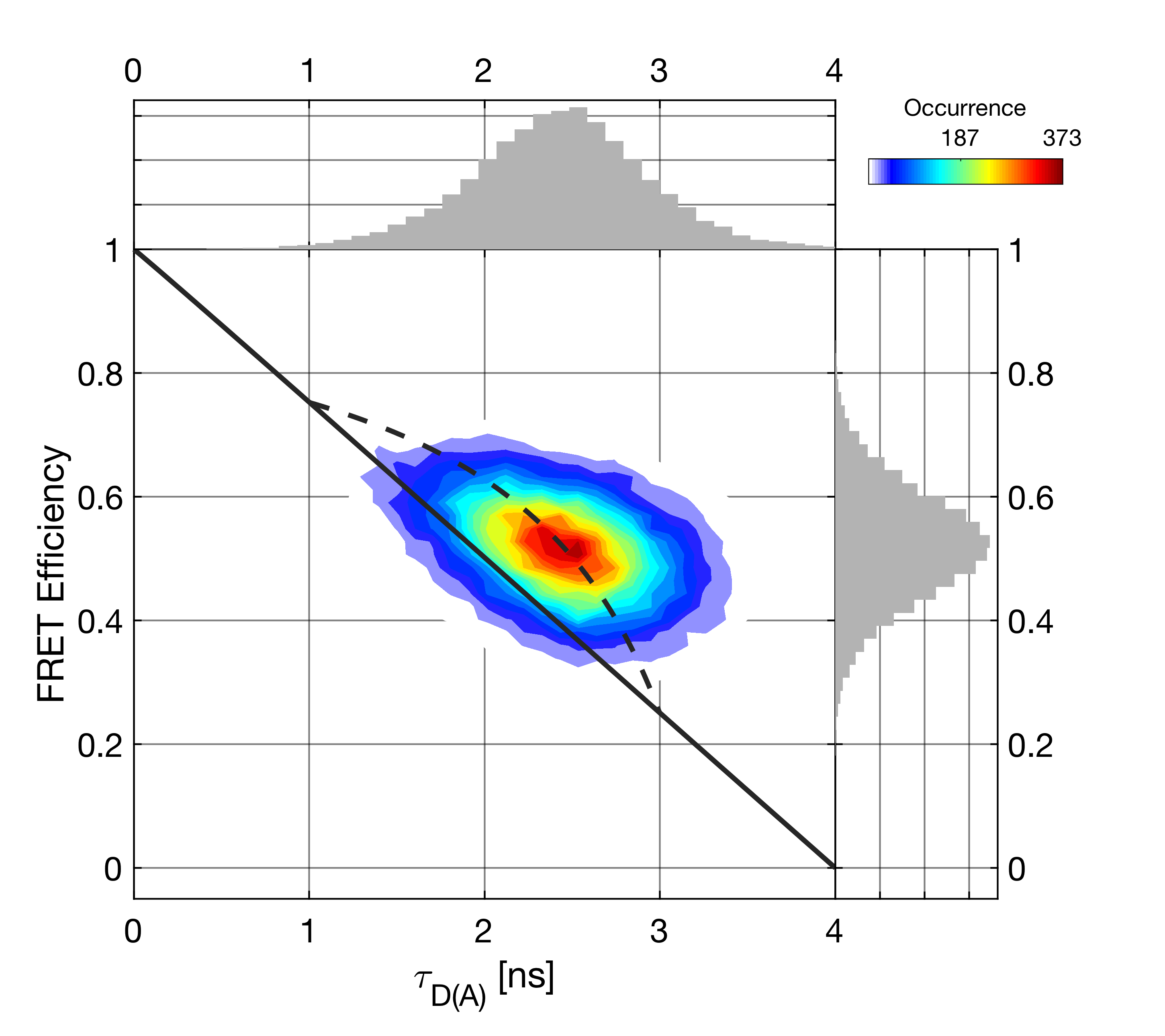
The E vs. \(\tau_{D(A)}\) plot indicates fast dynamics on the sub-millisecond timescale.

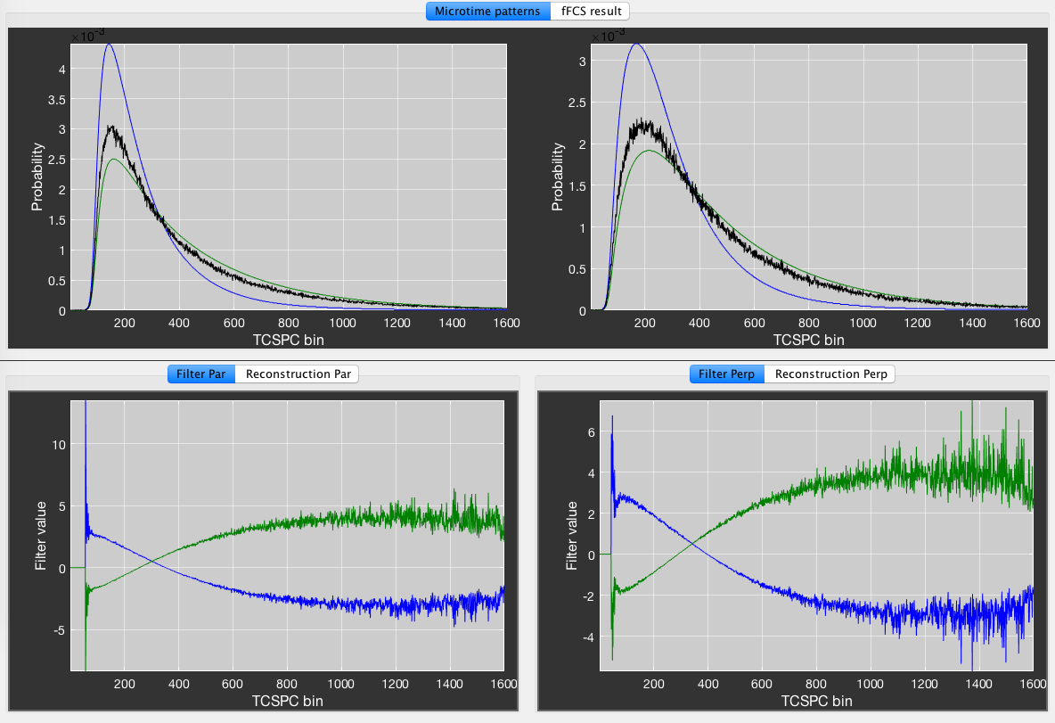
To perform the filtered-FCS analysis, we define two sub-species, representing the low and high FRET efficiency states by using thresholds of \(E < 0.35\) and \(E > 0.75\), respectively (Species 1 and Species 2). Click Plot Microtimes to plot the microtime patterns of the parent species (black) and Species 1 (green) and Species 2 (blue). Press the Calculate Filters button to define the filters for the two species. You can inspect the filters for the parallel and perpendicular channels in the plots at the bottom of the window. In the Reconstruction tab, inspect the measured (black) microtime pattern and the microtime pattern reconstructed from the decomposition (red) to judge the quality of the generated filters. Look for good agreement between the two patterns. If the two patterns do not agree well, usually a species that is present in the total measurement is not accounted for by any of the defined species (e.g. no background/scatter species included).

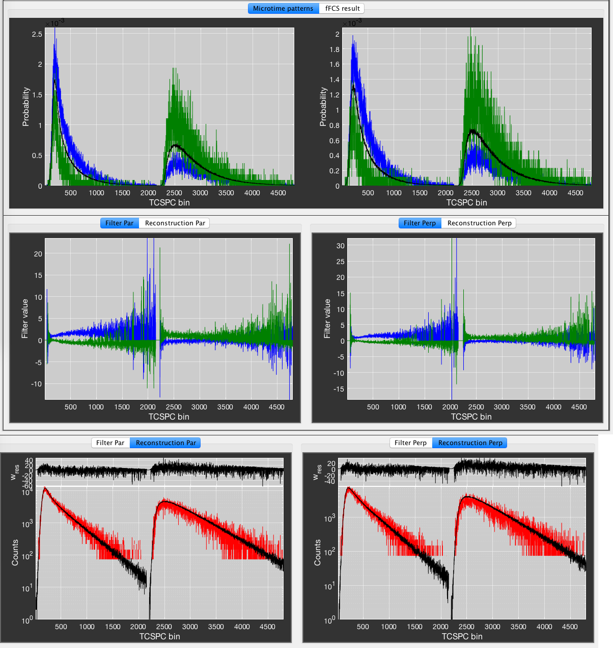
An example for fFCS analysis of the data in the previous figure. Blue species: E < 0.35, green species: E > 0.75.

Finally, click Do fFCS to perform the correlation analysis. The fFCS result will be plotted in the fFCS results tab. It will not be saved automatically. To save the result, click the Save result button to store the two autocorrelation and two cross-correlation functions in the folder of the .bur file.

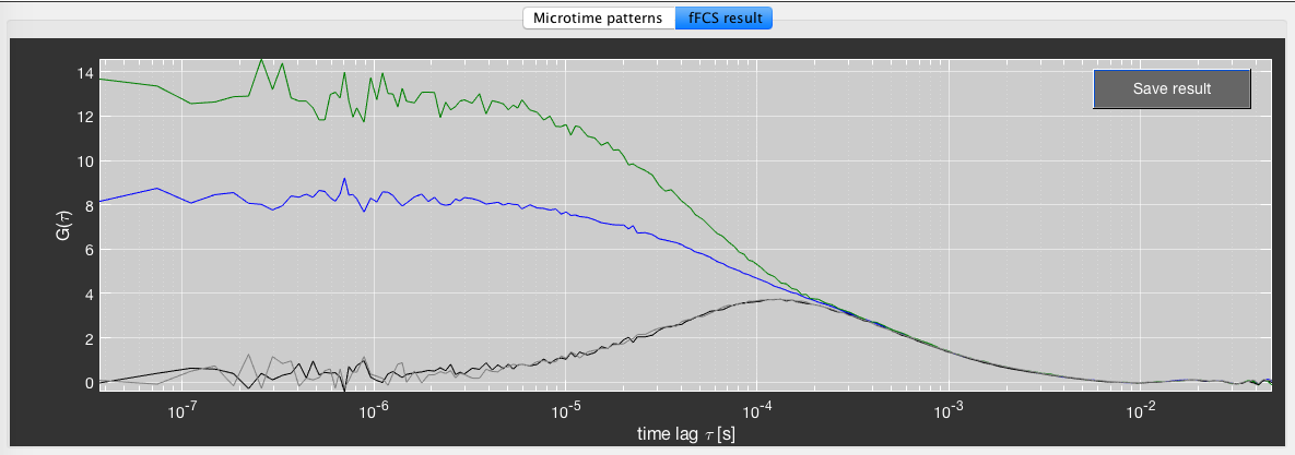
The result for the exemplary fFCS analysis.

There are several options to the fFCS analysis.

The fFCS mode allows you to select among the following approaches:

burstwise:

This mode will only use photons belonging to the selected bursts, identical to performing burstwise FCS analysis without the addition of a time window.

burstwise with time window:

This will add a time window around the selected bursts, identical to performing burstwise FCS analysis with the addition of a time window. It will use the time window specified in the FCS submodule. Since the addition of a time window will add more background signal, it is advised to include the scatter pattern to address the background contribution. An .aps file for the measurement, generated by checking the Save Total Photon Stream option upon performing of the burst analysis, is required.

continuous photon stream (with donor only):

This option will use the total measurement for the filtered-FCS analysis. As a consequence, all species present in the measurement need to be accounted for. Use the option without inclusion of a donor-only species only for samples that contain no or negligible amount of donor-only molecules. If donor-only molecules are present, usage of the option … with donor-only will determine the microtime pattern from the burst measurement using a stoichiometry threshold and include it in the analysis. Since the filtered-FCS analysis is not performed on the channel of acceptor emission after acceptor excitation (AA), there is no need to account for acceptor-only molecules. An .aps file, generated by checking the Save Total Photon Stream option upon performing of the burst analysis, is required. Since most of the signal will be originating from background, the inclusion of the scatter pattern as a species is required.

The option Include Scatter adds the stored scatter/background pattern as a third species. Enable this option when using the total measurement or including a large time window around the bursts.

Check Include FRET channel to stack the microtime histogram of the FRET channel with the donor channel. This increases the statistics by including FRET-induced acceptor photons, especially if very high FRET species are present.

To deal with noise microtime patterns cause by low statistics, e.g. if only a few bursts can be used to define a species, you can increase the TCSPC bin width, as is illustrated in the following figure. The reduced microtime resolution is only used for the filter calculation and does not affect the data in any other way.

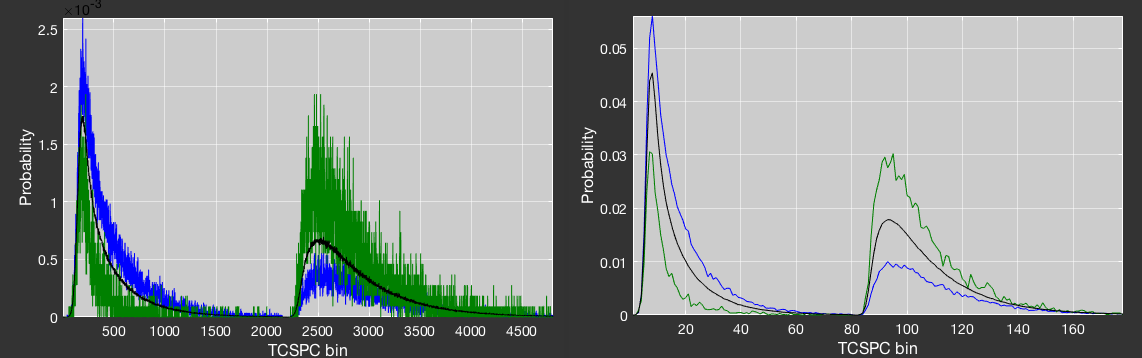
An example for increasing the bin width to deal with noisy microtime patterns.

Using synthetic microtime patterns

Another way to deal with statistics for the microtime patterns, or to include external microtime patterns, is to fit the fluorescence decay using TauFit and export the fitted microtime pattern. Note that it is required to use an anisotropy fit model to generate synthetic microtime patterns for both parallel and perpendicular decay. The usage of the FRET channel is not supported with synthetic microtime patterns, since there is currently no fit model for donor and acceptor decay simultaneously.

Synthetic microtime pattern generation in TauFit using an anisotropy fit model.

To load the .mi files, click the popupmenu of a species and select Load synthetic pattern…. Usage of synthetic patterns increases the quality of the filters through the reduced noise.

Example for using synthetic microtime patterns to generate filters for fFCS analysis.

Additionally, if the pure species are available in separate measurements, you can use the filtered-FCS module in PAM to export them as .mi files that can be loaded in BurstBrowser.

Exporting plots and data

Choosing the export location

By default, BurstBrowser saves exported files into the folder of the respective .bur file. If you are analyzing multiple data sets, it is convenient to collect all exported plots and data into a single folder. Disable the default behavior by unchecking the menu option Export -> Export to Current File Path. Choose a custom export path through Export -> Change Export Path. You can check the currently set export path under Export -> Current Export Path.

Note

The Export Path affects the save location of all exported plots and exported FRET histogram data. It does not affect the save location of PDA data or microtime patterns.

Exporting plots

Export of plots is implemented for all plots in the General and Lifetime tab, and are accessed via right-clicking the respective plots.

In the General tab, one-dimensional or two-dimensional plots can be exported individually. The Lifetime tab allows to export all lifetime-related plots in one figure (Export Lifetime Plots in the All tab), or the individual two-dimensional plots including the marginal parameter distributions in the Individual tab.

The resulting figures can be saved manually as any image format supported by MATLAB. Alternatively, you can have the program prompt you for saving when closing the figure by checking the Save file when exporting figure checkbox in the Options tab. The default output format is .png.

The Export all graphs button in the Options tab will automatically export the following graphs for the selected species: FRET efficiency vs. Stoichiometry, FRET efficiency, all lifetime-related plots and FRET efficiency vs donor lifetime.

Exporting data

FRET efficiency histogram export

FRET efficiency histograms can be exported to compare at a later time point or for further analysis in FCSFit. Exporting can be performed by right-clicking* the species in the Species List and selecting Export -> Export FRET Efficiency Histogram, which will save a .his file containing the FRET efficiency information of the selected bursts into the specified export folder. To perform export actions for multiple species at once, select the respective species and select the menu Export -> Export FRET Efficiency Histograms … -> for all selected species. Selecting for all selected files will instead export the last selected species for all files.

If the FRET efficiency histogram changes shape over the course of the measurement, you can export a time series to extract the kinetics from the data. Right-click the species in the Species List and select Export -> Export FRET Efficiency Histogram (Time Series). Specify the time window size in the following edit box. This will export FRET efficiency histogram of the measurement for non-overlapping time windows of the given size.

To compare previously exported .his files, select the menu Compare -> Compare FRET efficiency histograms from .his files and select the .his files you want to compare.

To globally analyze FRET efficiency histograms, load the .his files in FCSFit as described in the respective section.

Photon distribution analysis export

To analyze FRET efficiency data more quantitatively, it can be exported to PDAFit. The menu structure and export functionality is equivalent to FRET efficiency histogram export as described in the previous section. In addition to the menus, PDA export can be accessed by clicking the histogram button in the top row of the Species List.

PDA requires equivalent time bins for the FRET efficiency histogram analysis. The time bin size is specified in the Options tab in the Data Processing panel (default value: 1 ms). For kinetic analysis, it might be of interest to perform global analysis on the same data set exported with different time bin lengths. The edit box for specifying the time bin accepts standard MATLAB expressions to specify a list of time bins to export. Comma-separated lists of time bins (e.g 0.5,1,1.5,2) or range expression (e.g. 0.5:0.5:2) are accepted.

PDA data will always be exported into the folder of the respective .bur file and has the ending .pda.

Exporting microtime data

Microtime data of selected species can be exported by right-clicking the species and selecting Export -> Export Microtime Pattern. Exported microtime pattern (.mi extension) are used in PAM’s filtered FCS module to define pure species. If the patterns are too noisy due to low photon statistics, it is advisable to fit the microtime hisograms and use the fitted model function instead of the raw data. See the respective section in the TauFit manual for details.

Exporting to TauFit

Sub-ensemble TCSPC analysis on selected species can be performed by right-clicking and selecting Send selected Species to TauFit, or by selecting the fluorescence decay symbol in the top of the Species List. This will export the cumulative TCSPC histogram to TauFit. Note that data transfer is only implemented for single species and not integrated with multiselection. See the section on sub-ensemble TCSPC for more details.

Additional functionalities

Time window analysis

Dynamic interconversion between several FRET efficiency states on the sub-diffusion timescale will lead to averaging of the observed FRET efficiency dependant on the observation time. Right-click the species and select Time Window Analysis. This will plot the FRET efficiency histogram for time windows from 0.5 to 3 ms in intervals of 0.5 ms. Specify the minimum number of photons per time window to exclude time windows with low amount of photons and thus reduce shot noise in the histograms.

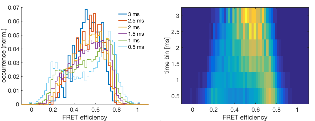
An example for identifying dynamics using time window analysis. The two distinct populations at low time windows are averaged at longer time windows.

Burst variance analysis

Given a FRET distribution broader than the expected shot-noise distribution, Burst variance analysis (BVA) can be used to distinguish between multiple static components or multiple interconverting states. Right-click the species and select Burst Variance Analysis. This will plot the observed and expected standard deviation of the proximity ratio for each burst and the corresponding confidence interval (CI) against the selected X-axis. Each burst will be segmented into consecutive windows of a specified number of photons. The standard deviation is binned using a width of 0.05 along the X-axis. Specify a threshold for the number of bursts per bin to increase statistical power by excluding bins with a low amount of bursts. The CI considers the sampling distribution of standard deviations expected for the number of photon windows by using a Monte Carlo approach. Specify the sampling number (i.e. number of simulations) to get a binomial distribution of standard deviations (e.g. 100 for a valid CI or 1 for a fast calculation). Specify the CI \(\alpha\) to adjust the upper-tail CI (i.e. low \(\alpha\) value for higher confidence interval and high \(\alpha\) value for lower CI). Select either the proximity ratio or FRET efficiency as the X-axis (note: for FRET efficiency the expected standard deviation has an oval shape).

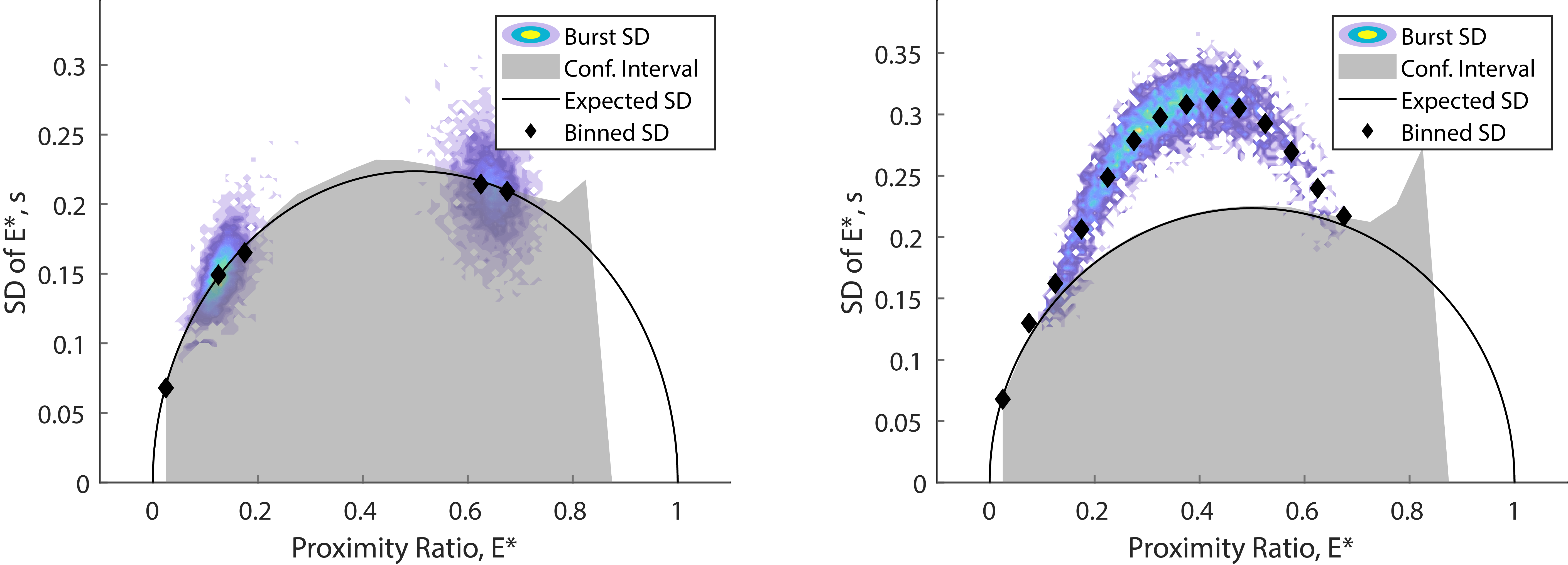
An example for identifying dynamics using burst variance analysis. Standard deviation values clustering around the expected standard deviation indicate static FRET (left panel) whereas bursts with standard deviation values significantly above the confidence interval indicate within-burst dynamics (right panel).

Working with large data sets

BurstBrowser offers functionality to work with multiple files simultaneously, such as synchronizing correction factors and cut states. Additionally, many export functionalities work with multiselection.

To load multiple measurements from a single folder, select File -> Load New Burst Data (shortcut ctrl+N) and select the measurements to load. Add burst files to the currently loaded files by selecting File -> Add burst data. To easily load many measurements at once, use the File -> Load New Burst Files from Subfolders menu. This will search through all subfolders of the selected folder and load any .bur files found.

To keep track of files that belong together, you can group them into a database. In the Database tab, select Add files to database to add new files to the current database. Use Append loaded files to database to add all loaded to the current database. Create database from folder has the same functionality as the option to load burst files from subfolders. Individual files can be removed from the database by selecting them in the list and using the del key. To load a selection of files from the database, use enter. Databases can be saved as .bdb files and reloaded at a later time point. Additionally, BurstBrowser remembers the last used database, so you can continue working on the last dataset immediately.

In addition, BurstBrowser keeps track of the last 20 loaded files in the File History. Use enter to load selected files from the File History, and del to remove files.

Saving the analysis state

Save the edits to all currently loaded files by selecting the menu File -> Save Analysis State (shortcut ctrl+S). This will save the cut state and corrections/parameters. Any fit lines in the lifetime plots, correction plots or the state of filtered-FCS analysis will however not be remembered.

Hint

To avoid loss of data, enable the Ask for saving when closing program checkbox in the Options tab. This will prompt you to save the analysis state when closing BurstBrowser. Select Discard to close the program without saving the changes, and Cancel to abort the closing progress and continue with the analysis.

Keeping notes

BurstBrowser offers an internal Notepad which you can use to keep temporary notes. Open it using the menu Notepad or by shortcut ctrl+T. The notes are saved in the currently selected PAM profile and kept between sessions. You can save the contents of your current notepad as a .txt file by right-clicking the text and selecting Save contents.

---

Table of parameters in BurstBrowser

List of correction factors

\(\gamma\)-factor:

Accounts for differences in quantum yield \(\Phi\) and detection efficiency \(g\). Given by

\(\gamma = \frac{\Phi_Ag_A}{\Phi_Dg_D}\)

\(\beta\)-factor:

Accounts for differences in extinction coefficient \(\epsilon\) and incident laser power \(I\) in alternating excitation at the given excitation wavelength \(\lambda_{\mathrm{exc}}\), as defined in [Lee2005]:

\(\beta = \frac{\epsilon_A^{\lambda_{\mathrm{exc}}^A}I_A}{\epsilon_D^{\lambda_{\mathrm{exc}}^D}I_D}\).

crosstalk/\(ct\):

Fraction of donor signal that is detected in the acceptor channel.

direct excitation/\(de\):

Fraction of acceptor signal originating from direct excitation of the acceptor by the donor excitation laser. This correction is performed based on the signal of the acceptor after acceptor excitation (RR) and is thus dependent on the acceptor laser power.

\(G\)-factor:

Corrects differences in detection efficiencies \(g\) of parallel and perpendicular polarization. Given by

\(G=\frac{g_{\perp}}{g_{\parallel}}\)

\(l_1\)/\(l_2\):

Factors accounting for polarization mixing caused by the high N.A. objective lens. See definition of anisotropy.

BG:

Background count rate of the given channel in kHz. Photon counts \(T\) are corrected for background contribution based on the burst duration \(T\) by

\(N_{\mathrm{cor}}=N-BG*T\)

---

List of burst-wise parameters

FRET efficiency:

Corrected FRET efficiency calculated using

\(E = \frac{GR-ct*GG-de*RR}{\gamma*GG + GR-ct*GG-de*RR}\)

with background-corrected photon counts.

Stoichiometry:

Corrected labeling stoichiometry calculated using

\(S =\frac{\gamma*GG+GR-ct*GG-de*RR}{\gamma*GG+GR-ct*GG-de*RR+\beta*RR}\)

with background-corrected photon counts. \(\beta\)-factor correction is optional and can be disabled using the checkbox (Ref).

Proximity ratio:

Uncorrected FRET efficiency based on the raw signal

\(PR=\frac{GR}{GG+GR}\)

Stoichiometry (raw):

Uncorrected labeling stoichiometry based on the raw signal

\(S=\frac{GG+GR}{GG+GR+RR}\)

Anisotropy D/A:

Steady-state fluorescence anisotropy of donor or acceptor fluorophore calculated by

\(r_{\mathrm{ss}}=\frac{G*I_\parallel-I_\perp}{G(1-3*l_2)I_\parallel+(2-3*l_1)I_\perp}\)

Lifetime D/A [ns]:

Burst-wise fluorescence lifetime of donor or acceptor fluorophore determined from a maximum-likelihood estimator using a constant background contribution. See [Maus2001] for details on the MLE.

Mean macrotime [s]:

Burst-wise mean macrotime (arrival time) in seconds with respect to the start of the measurement.

Number of photons:

Uncorrected number of photons per burst for selected channel.

Duration [ms]:

Duration of burst given by the time interval between first and last photon, determined from all photons or the selected channel.

Count rate [kHz]:

Burst-wise average count rate in kHz calculated from total number of photons and burst duration.

|TGX-TRR| filter:

Difference in mean macrotime between the combined photons after donor excitation (GX) and the photons after acceptor excitation (RR), normalized to the burst duration. This filter is sensitive to bleaching of donor or acceptor dye. See [Kudryavtsev2012] for more details.

|TGG-TGR| filter:

Defined analogously to |TGX-TRR| filter, but between donor and FRET channel. This filter is sensitive to dynamic fluctuations between FRET states. See [Kudryavtsev2012] for more details.

ALEX 2CDE filter:

This filter sensitive for fluctuations of the signal after donor excitation with respect to the signal after acceptor excitation, and can thus be used to filter donor or acceptor blinking and bleaching events. See [Tomov2012] for details of filter calculation.

FRET 2CDE filter:

Similar to the ALEX 2CDE filter, this filter is sensitive to relative fluctuations of the donor and FRET signal, and can thus be used to detect dynamic interconversion between different FRET states. See [Tomov2012] for details of filter calculation.

FRET efficiency (from lifetime):

FRET efficiency determined from burst-wise lifetime \(\tau_{D,A}\) and specified donor-only lifetime \(\tau_{D,0}\) using

\(E = 1-\frac{\tau_{D,A}}{\tau_{D0}}\)

Distance (from intensity/from lifetime) [Angstrom]:

Calculated distance from burst-wise FRET efficiency (either determined from intensity or lifetime) using the given Förster radius \(R_0\):

\(R = R_0\left(\frac{1}{E}-1\right)^{-1/6}\)

[Kudryavtsev2012]

(1, 2) Kudryavtsev, V. et al. Combining MFD and PIE for Accurate Single-Pair Förster Resonance Energy Transfer Measurements. ChemPhysChem 13, 1060–1078 (2012).

[Botev2010]

Botev, Z. I., Grotowski, J. F. & Kroese, D. P. Kernel density estimation via diffusion. The Annals of Statistics 38, 2916–2957 (2010).

[Lee2005]

(1, 2) Lee, N. K. et al. Accurate FRET Measurements within Single Diffusing Biomolecules Using Alternating-Laser Excitation. Biophys J 88, 2939–2953 (2005).

[Kalinin2010]

(1, 2) Kalinin, S., Valeri, A., Antonik, M., Felekyan, S. & Seidel, C. A. M. Detection of structural dynamics by FRET: a photon distribution and fluorescence lifetime analysis of systems with multiple states. J. Phys. Chem. B 114, 7983–7995 (2010).

[Laurence2007]

Laurence, T. A. et al. Correlation spectroscopy of minor fluorescent species: signal purification and distribution analysis. Biophys J 92, 2184–2198 (2007).