FCSFit

Contents

• FCSFit
  • Data handling and loading
    • Saving the analysis state
  • Fitting models and algorithms
    • Fit models
    • Fitting procedure
  • Additional settings and exporting
  • Alternate mode for global fitting of FRET efficiency histograms

Fitting of FCS data can be accessed from the PAM main window by clicking on Advanced Analysis -> FCSFit or from the command window by typing in FCSFit.

The upper part of the window is dedicated for displaying the FCS data, fits and corresponding residuals. In the lower part of the window the user can set the fit parameters and other fitting and display settings.

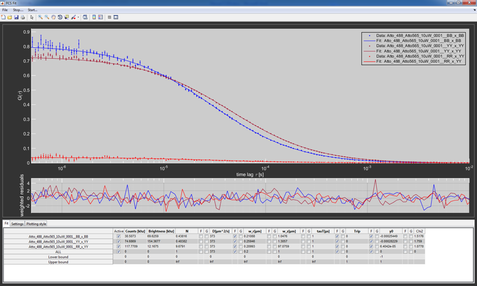
FCSFit main gui

Data handling and loading

Currently, the program only supports files created with PAM, both based on MATLAB files (.mcor) and text files (.cor).

To load new files, got to File -> Load New Files or File -> Add Files. The former clears previously loaded files and load the new ones, while the later adds new files to the loaded ones. All loaded files are listed in the table and the bottom. Individual files can be removed by clicking on the Remove checkbox in the Plotting Style tab.

The raw correlation data is accessible from the command line via the global variable FCSData, and the fits and other processed parameters are stored in the global variable FCSMeta.

Saving the analysis state

The analysis state can be saved as a session (.fcs file) under File -> Save FCSFit Session. This will save all fitted parameters including global and fixed flags, the loaded model function, all settings and the visualization state (line types, curve colors…). Load a previous session using File -> Load FCSFit Session.

Fitting models and algorithms

Fitting in FCSFit is not based on hard coded fit models but instead uses models stored in text files (standard .txt). This allows users to easily create new models and modify old ones without having to change the code itself, especially useful for a compiled program.

Fit models

FCSFit uses text based fit models. A simple example of the structure of a model is shown here:

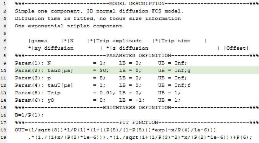
Example model text file

Each model file consists of four segments. The headers of the segments are needed for the program to recognize the individual parts and should not be modified.

Model description:

This part is not used by the program itself but is used as a description for the user to understand the purpose and outline of the fit.

Parameter definition:

In this section the different parameters used for the fit are defined and initial values set. The nth parameter is defined by Param(n):, followed by the name of the parameter displayed in FCSFit (do not use spaces in the name as they are used as separators). The next settings in order are the initial value, the lower and the upper limits. At the end you can use g or f to the set the parameter to global or fixed during initialization of the fit. The equal signs and semicolons are essential as the program searches for them as separators between the entries.

Brightness definition:

The program uses this part to calculate the molecular brightness. Generally, the brightness is defined as 1/N, but can be more complex for other models. Use standard MATLAB nomenclature to define this function and terminate it with a semicolon.

Fit function:

Here the actual function used for fitting is defined. The individual parameters are abbreviated as P(n). Use standard MATLAB nomenclature to define the function. Multiline entries are possible. In such a case use simple line breaks and not the ... used in MATLAB scripts and functions.

Fitting procedure

When starting FCSFit, the model used during the last session is pre-loaded. A different fit function can be selected via File -> Load Fit Function. The standard folder for this is the models sub-folder of PAM.

The file names and the fit parameters defined in the model are shown in the table in the Fit tab.

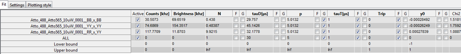
The fit table

The different rows correspond to the individual files. The last three rows are used to set parameters for all files, the lower and the upper bounds, in order.

The first column after the filenames is used to (de-)activate individual files to include them in or exclude them from the fitting and displaying procedure. The following column shows the average count rate of the file. For cross-correlation it is the sum of both channels. This is followed by the molecular brightness, calculated from the brightness defined in the model time the count rate. The other columns correspond to the different fit parameters with three columns each. The first is an editbox that contains the actual value. The other two are checkboxes used to either fix a parameter (F) or to globally link it between all files (G). The very last column represents the \(\chi^2_\textrm{red.}\) of the fit.

For the actual fitting, FCSFit uses the standard MATLAB least-square curve fitting algorithm (lsqcurvefit). Only the data-points displayed in the upper plot (defined in the Settings tab) are used for fitting. When no variables are linked globally, each file is fit individually. The free parameters are used for the fit, while the fixed variables are given to the function as additional data to calculate the functions. For a global fit, the variables and fit-functions are concatenated and a single fit is executed. After the fit is finished, confidence intervals are calculated and the plots and tables updated.

Additional settings and exporting

With the Plotting Style tab the user can change the appearance of the plotted data and fits. The Settings tab contains contains a variety of parameters for fitting and displaying, most notably the time range to be displayed and used for fitting (Borders), whether or not to use weights (Use weights) and other fit related settings. Furthermore, it contains general setting for exporting the curves to a new MATLAB window.

The curves can be exported to a new figure or the data can be exported to the MATLAB command line by right clicking the plot and selecting the appropriate function. Additionally, the Copy Results to Clipboard button copies the fit parameters to the clipboard so they can be parsed into standard programs like excel of origin.

Alternate mode for global fitting of FRET efficiency histograms

FCSFit can also be used to fit FRET efficiency histograms exported from BurstBrowser (see Exporting FRET efficiency histograms). Upon file loading, select “FRET efficiency data from BurstBrowser” to load .his files. Currently, models are available for fitting of normal and \(\beta\)-distributions. Note that the \(\beta\)-distribution is only defined in the interval [0,1].

If Plot errorbars is checked, the data is shown as line plot with error bars. Error bars are determined assuming Poissonian counting statistics for the histogram, i.e. by \(\sigma = \sqrt{N}\) where N is the number of counts. If this option is unchecked, data will be shown as stair plots.

FRET efficiency data can be rebinned by changing the bin size (default bin size: 0.01). Choose an appropriate value depending on the sampling of the FRET efficiency histogram.

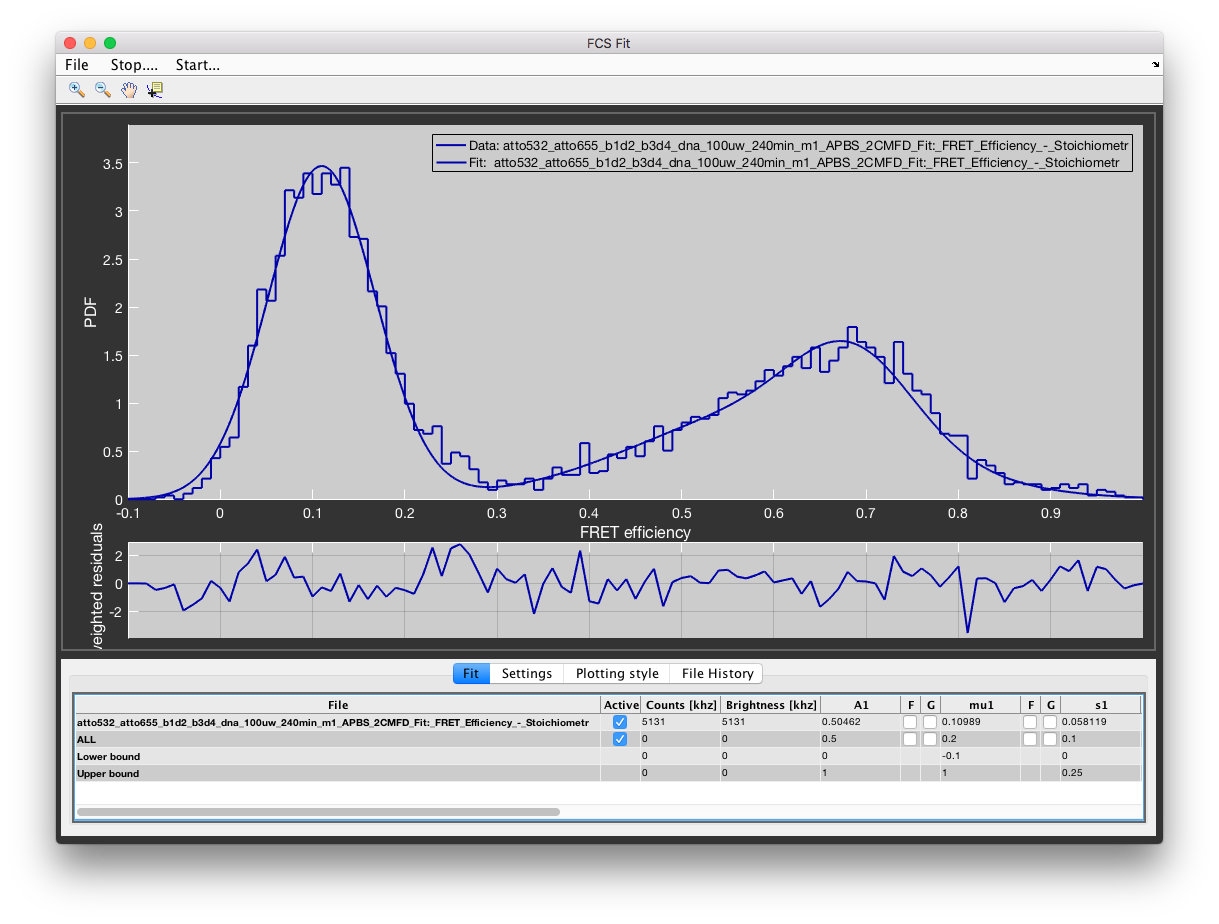
FRET efficiency histogram analysis in FCSFit using Gaussian distributions