MIAFit

Contents

• MIAFit
  • Data handling and loading data
  • Fitting models and algorithms
    • Fit models
    • Fitting procedure
  • Data display
  • Additional setting and exporting

Fitting of 2D and 3D correlation data can be accessed from the PAM main window by clicking on Advanced Analysis -> MIAFit or from the command window by typing in MIAFit.

The program work in many ways identical to FCSFit with small differences in displaying the data. The upper part of the window is dedicated for displaying the correlation data, either as 1D on-axis plots for all files, or as a 2D representation for a single file. In the lower part of the window the user can set the fit parameters and other fitting and display settings.

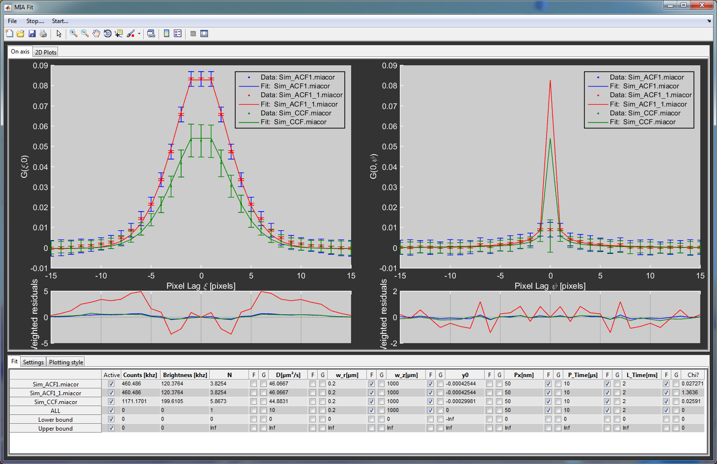
The main GUI of MIAFit.

Data handling and loading data

Currently, the program only supports files created with PAM, both based on MATLAB files (.miacor) and TIFF files with additional information added in an info file. A third type are STICS files (.stcor) that treat the different lags as individual files.

To load new files, got to File -> Load New Files or File -> Add Files. The former clears previously loaded files and load the new ones, while the later adds new files to the loaded ones. All loaded files are listed in the table and the bottom. Individual files can be removed by clicking on the Remove checkbox in the Plotting Style tab. Only one STICS file can be loaded at once and all previous files will be cleared.

The raw correlation data is accessible from the command line via the global variable MIAFitData, and the fits and other processed parameters are stored in the global variable MIAFitMeta.

Fitting models and algorithms

Fitting in MIAFit is not based on hard coded fit models but instead uses models stored in text files (.miafit). This allows users to easily create new models and modify old ones without having to change the code itself, especially useful for a compiled program.

Fit models

MIAFit uses text based fit models. An example of the structure of a model is shown here:

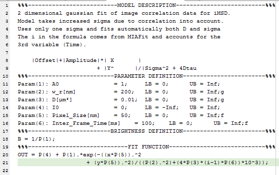
An example fit model for MIAFit.

Each model file consists of four segments. The headers of the segments are needed for the program to recognize the individual parts and should not be modified.

Model description:

This part is not used by the program itself but is used as a description for the user to understand the purpose and outline of the fit.

Parameter definition:

In this section the different parameters used for the fit are defined and initial values set. The nth parameter is defined by Param(n):, followed by the name of the parameter displayed in MIAFit (do not use spaces in the name as they are used as separators). The next settings in order are the initial value, the lower and the upper limits. At the end you can use g or f to the set the parameter to global or fixed during initialization of the fit. The equal signs and semicolons are essential as the program searches for them as separators between the entries.

Brightness definition:

The program uses this part to calculate the molecular brightness. Generally, the brightness is defined as 1/N, but can be more complex for other models. Use standard MATLAB nomenclature to define this function and terminate it with a semicolon.

Fit function:

Here the actual function used for fitting is defined. The individual parameters are abbreviated as P(n) and the variables are x and y. The additional variable i can be used for 3D correlation data. This value is given by the file number and is mostly used for STICS data. Keep in mind that the first file of .stcor data (i.e. i=1) contains the zero lag correlation. Use standard MATLAB nomenclature to define the function. Multiline entries are possible. In such a case use simple line breaks and not the … used in MATLAB scripts and functions.

Fitting procedure

When starting MIAFit, the model used during the last session is pre-loaded. A different fit function can be selected via File -> Load Fit Function. The standard folder for this is the models sub-folder of PAM.

The file names and the fit parameters defined in the model are shown in the table in the Fit tab.

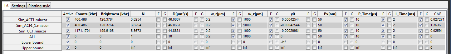
The fit parameter table of MIAFit.

The different rows correspond to the individual files. The last three rows are used to set parameters for all files, and the lower and the upper bounds, in order.

The first column after the filenames is used to (de-)activate individual files to include them in or exclude them from the fitting and displaying procedure. The following column shows the average count rate of the file. For cross-correlation it is the sum of both channels. This is followed by the molecular brightness, calculated from the brightness defined in the model time the count rate. The other columns correspond to the different fit parameters with three columns each. The first is an editbox that contains the actual value. The other two are checkboxes used to either fix a parameter (F) or to globally link it between all files (G). The very last column represents the \(\chi^2_{\textrm{red.}}\) of the fit.

For the actual fitting, MIAFit uses the standard MATLAB least-square curve fitting algorithm (lsqcurvefit) and linearizes the data. Only the data-points displayed in the upper plot (defined in the Settings tab) are used for fitting. When no variables are linked globally, each file is fit individually. The free parameters are used for the fit, while the fixed variables are given to the function as additional data to calculate the functions. For a global fit, the variables and fit-functions are concatenated and a single fit is executed. After the fit is finished, confidence intervals are calculated and the plots and tables updated. For auto-correlation curves, the (0,0) spatial lag point contains the noise peak. Furthermore, some cameras show strong artifacts for a line correlation. Therefore it is possible to omit either the center point of the whole line from the fitting algorithm in the Settings tab.

Data display

Displaying 2D data is much more complicated that for just a single dimension. MIAFit has therefore two different ways of visualization. The first shows the on-axis correlation of all loaded files with the corresponding error bars, fits and residuals. The left side shows the fast and the right side the slow axis for RICS data. The second display option shows the full correlation as a surface plot for a single file. Next to it, the user can display the fit, the residuals or a combination of both.

Additional setting and exporting

With the Plotting Style tab the user can change the appearance of the plotted data and fits. The Setting tab contains contains a variety of parameters for fitting and displaying, most notably the time range to be displayed and used for fitting (Borders), whether or not to use weights (Use weights), to omit the center point (Center), the whole y=0 line (Line), a specified number of lines (Points) and other fit related settings. Please be advised that data in which several points have to be omitted from the fitting might be compromised. Furthermore, it contains general setting for exporting the curves to a new MATLAB window. The curves can be exported to a new figure or the data can be exported to the MATLAB command line by right clicking the plot and selecting the appropriate function. Additionally, the Copy Results to Clipboard button copies the fit parameters to the clipboard so they can be parsed into standard programs like Excel of Origin.