TauFit
Contents
TauFit is the central TCSPC module of PAM, dedicated to the analysis of fluorescence intensity decays and time-resolved anisotropy. The following analysis methods are available:
- Tail fitting of fluorescence decays and time-resolved anisotropy
- Reconvolution fitting of fluorescence decays using:
- Single, bi- or triexponential model
- Distribution of donor-acceptor distances
- Time-resolved anisotropy model
- Simulation of \(\kappa^2\)-distributions from fundamental and residual anisotropies
TauFit integrates with both PAM for ensemble-TCSPC analysis and BurstBrowser for burst-selective sub-ensemble TCSPC analysis of species.
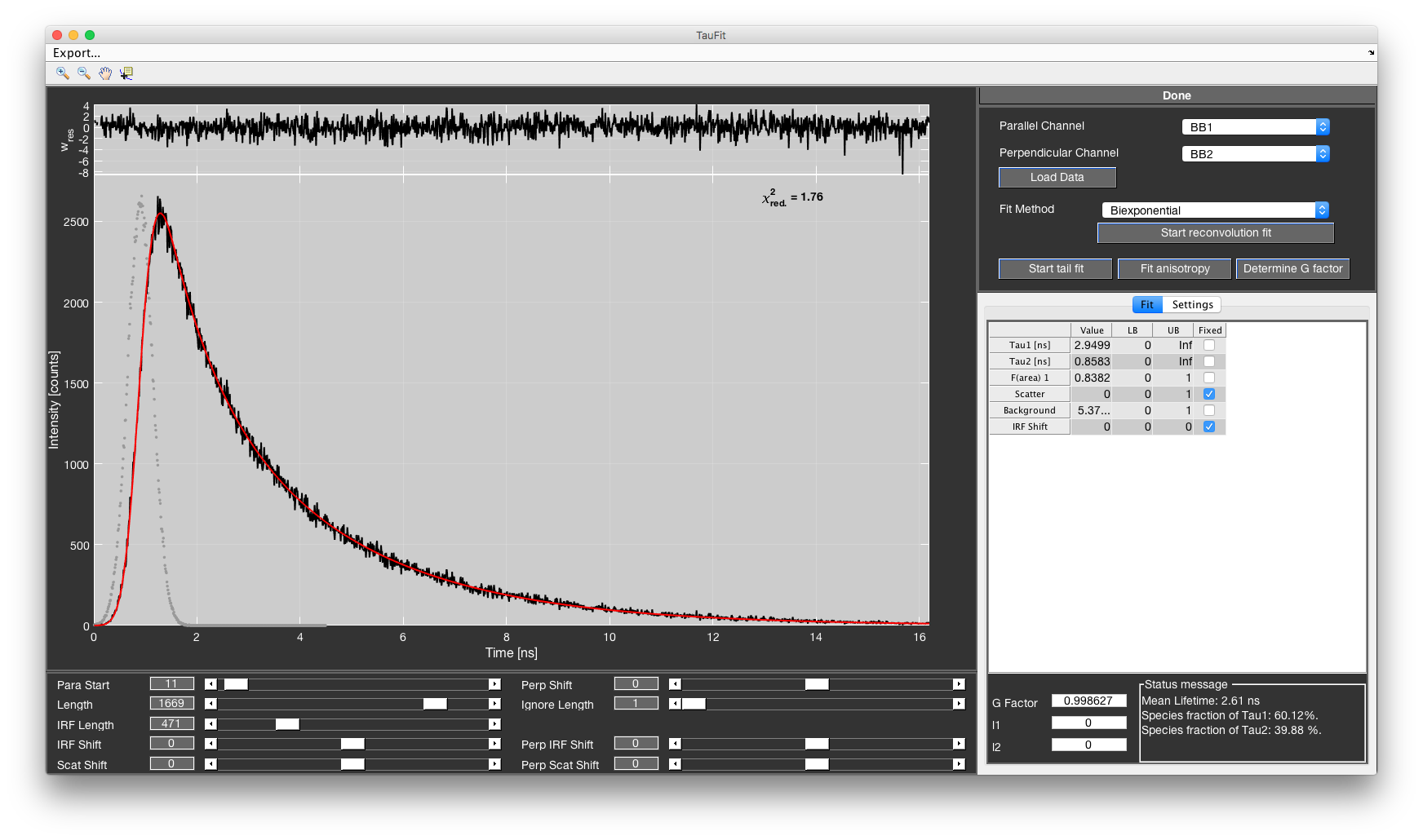
TauFit’s main GUI.
Data loading
From PAM (ensemble-TCSPC)
The selection GUI.
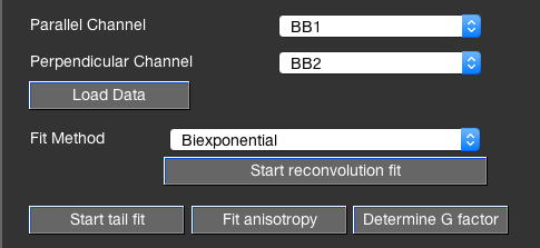
TauFit directly accesses the data loaded into PAM via the defined PIE channels. To load fluorescence decay data into TauFit from PAM, choose the PIE channels for the parallel and perpendicular fluorescence signal using the popupmenus and click Load Data. If no polarized detection is used, simply select the same channel twice.
From BurstBrowser (subensemble-TCSPC)
To analyze the fluorescence decay of a species from a burst measurement, you can directly export it from BurstBrowser as described in the respective section in the BurstBrowser manual.
From intermediate file format .decay
PAM allows to export the microtime decays of a raw data file into a processed .dec file as described in the respective section of the PAM manual. To load .dec files, select File -> Load decay data (.dec). Note that this will put TauFit into external data mode, disabling interaction with the currently loaded data in either PAM or BurstBrowser. Close TauFit and open a new instance to re-enable the default mode.
Aligning the data
Main plot

The main plot shows the raw fluorescence decay data of the selected PIE channels, using red for the parallel channel and blue for the perpendicular channel. The respective instrument response functions (IRF) are plotted as dotted lines. Additionally, the scatter patterns for both channels are indicated as dotted gray lines. If the ignore slider is used, a vertical black line indicates the start point of the data that is consider for the goodness-of-fit calculation.
Alignment sliders
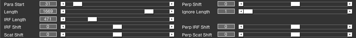
The alignment sliders.
An important step when fitting fluorescence decays obtained on avalanche photodiodes is the alignment of the channels with respect to each other. The sliders should be used in the proposed order:
- Start: Global start of the data range with respect to the PIE channel range, i.e. a value of 10 omits the first 10 TCSPC bins.
- Length: Total length of the data range.
- Perp Shift: Shift of the perpendicular decay with respect to the parallel decay. Affects both the data and the IRF pattern.
- IRF Length: Length of the IRF pattern to be used for reconvolution fitting.
- IRF Shift: Shift of the IRF pattern with respect to the fluorescence decay.
- Perp IRF Shift: Alignment of the IRF in the perpendicular channel with respect to the parallel channel IRF.
- Scat Shift: Shift of the scatter pattern with respect to the fluorescence decay.
- Perp IRF Shift: Alignment of the scatter pattern in the perpendicular channel with respect to the parallel channel scatter pattern.
- Ignore Length: Can be used to ignore a part of the data range for the calculation of the \(\chi^2_{\textrm{red.}}\), while still using the omitted data range for reconvolution.
Generally, the IRF pattern has to be shifted to accurately fit the data using the reconvolution approach. This is caused by countrate dependent timing shifts of the APDs, since IRF and TCSPC measurement are usually performed at different count rates. It can be difficult to correctly assign the shift of the IRF pattern with respect to the fluorescence decay. The user can instead supply a range of IRF shifts and let TauFit find the optimal value (see the description of the fit table).
Correction factors
For accurate fluorescence lifetime and anisotropy analysis, a few correction factors have to be known. Most important for lifetime analysis is the so-called G-factor, accounting for differences in the detection efficiency \(\eta\) between the parallel and the perpendicular detection channel.
G can be determined from the relative intensity levels from a measurement of an uncorrelated light source, i.e. a fluorescent dye with a short rotational correlation time. One can either directly take the ratio of the fluorescence signal at large lag time, or calculate G from the residual anisotropy \(r_\infty\) of the dye measurement (see Time-resolved anisotropy fitting). G is the given by:
The button Determine G factor can be used to automatically determine G using the described method. The data range should be selected as described for tail fitting or time-resolved anisotropy analysis using the Ignore Length slider.
Additionally, anisotropy measurements with high numerical aperture objectives are subject to depolarization due to polarization mixing [Koshioka1995]. This causes a decrease of the measured anisotropy and is accounted for by the correction factors \(l_1\) and \(l_2\).
Basic data analysis
Tail fitting
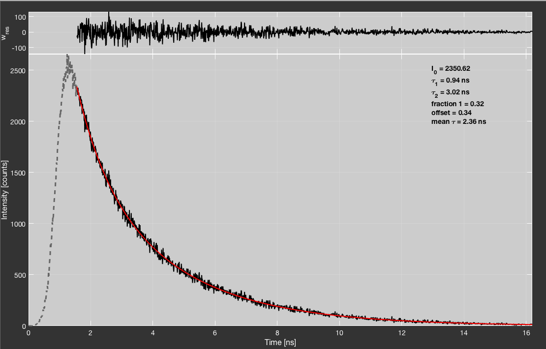
Tail fitting using a biexponential model function.
For a quick determination of the fluorescence lifetime, a single or biexponential or triexponential tail fit of the fluorescence decay can be performed. The parallel and perpendicular channels should be aligned properly. Additionally, the initial rise of the fluorescence decay should be excluded either by using the Para Start or the Ignore Length slider. The fit result is displayed in the top right corner of the plot.
The fit model is given by:
For fitting, the parallel and perpendicular fluorescence decays are combined such that the anisotropy information is canceled out.
Tail fitting uses weighted residuals if specified in the options (Use weighted residuals).
Intensity vs. species fraction in TCSPC
When using multi-exponential fit models to describe TCSPC data, it is important to note that the obtained fractions \(\alpha_i\) give the amplitudes at time t = 0 and are proportional to the number of molecules of the respective lifetime. However, the intensity contribution of a species to the fluorescence decay is proportional to the area of the curve, given by \(A_i = \tau_i \alpha_i\). The average lifetime of a multi-exponential is calculated based on the intensity fractions \(f_i\) given by:
The average lifetime is then given by:
This value is reported in the Status Message box in the bottom right, along with the respective intensity fractions.
On the contrary, the value of:
is proportional to the area under the curve and thus the steady-state intensity. See [Lakowicz2007] for more details.
Time-resolved anisotropy fitting
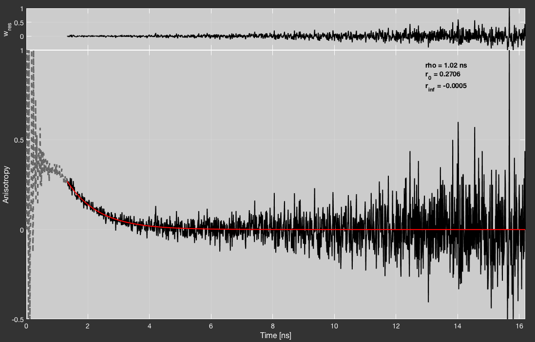
Time-resolved anisotropy fitting.
Similar to tail fitting of fluorescence decays, the time-resolved anisotropy can be analyzed using basic fitting. The anisotropy decay is calculated using:
The standard model function is based on the wobbling-in-cone approximation, which assumes that the fluorophore’s rotation is restricted by the attachment to the biomolecule. It is given by:
where \(r_0\) is the fundamental anisotropy of the fluorophore, \(\rho\) is the rotational correlation time describing the local motion, and \(r_\infty\) is the residual anisotropy due to the slow rotational movement of the biomolecule on a timescale larger than the fluorescence lifetime. If the rotation of the biomolecule \(\rho_p\) is faster, it can be described by an additional exponential term:
The biexponential fit model is available by right clicking the Fit anisotropy button.
Additionally, a model called “dip-and-rise” can be fitted. This model assumes two independent species with different fluorescence lifetimes and rotational behavior, where each component shows a mono-exponential anisotropy decay and single-component fluorescence lifetime. A “dip-and-rise” behavior is often observed for cyanine dyes, where a change in the rotational freedom is connected to the fluorescence lifetime, an effect known under the name PIFE for protein induced fluorescence enhancement. Generally, steric hindrance limits the cis-trans isomerization rates, resulting in a longer fluorescence lifetime, whereas the sterically free dyes show a short fluorescence lifetime. A superposition of both species will result in the “dip-and-rise” anisotropy decay, since the average anisotropy depends on the relative contributions of the two species. The fast-rotating low-anisotropy species contributes at small lag times, causing the anisotropy to decline fast initially. At longer lag times, mainly the slow-rotating high-anisotropy species contributes to the fluorescence signal, causing the anisotropy to rise again.
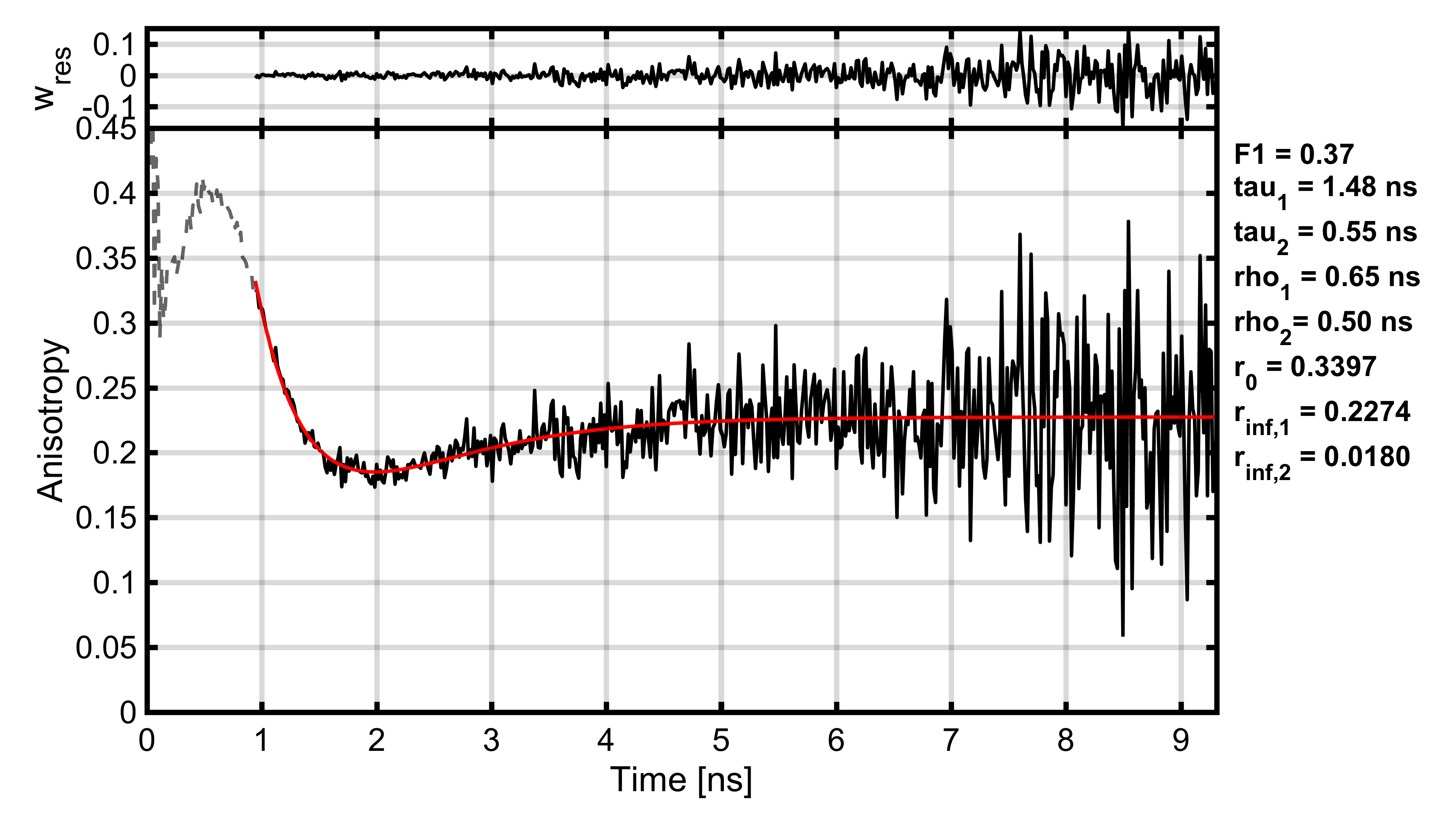
“Dip-and-rise” behaviour of Cy3 labeled sample.
The model function is given by:
Here, the amplitude of species 1 \(A_1(t)\) is given by:
The model assumes identical fundamental anisotropy \(r_0\) for both species. The returned parameter \(F_1\) is the fraction of species 1 given by:
Reconvolution fitting
Reconvolution fitting uses the experimentally obtained instrument response function (IRF) to convolute the model function:
Here, \(\ast\) denotes the convolution operation. If polarized detection is used, the anisotropy-free fluorescence decay is constructed as described above. The IRF of the combined channel is then approximated in the same manner.
The Convolution Type can be changed in the Settings tab. Linear convolution performs convolution without periodicity. If the selected PIE channels spans the total available microtime range, i.e. the decay pattern is periodic, circular convolution should be used.
Fit table
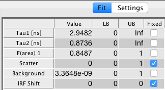
The fit parameter table.
The fit table shows the parameters of the currently selected Fit Method. Initial parameter values and lower and upper boundaries (LB, UB) can be specified here. Additionally, parameters can be fixed.
The IRF Shift parameter is a special case. If it is unfixed, the fit will iterate over a range of IRF shift values given by the specified center value and lower/upper bound, i.e. from Shift-LB:1:Shift+UB, and perform the fit routines at those shift values. The goodness of fit is compared between all fits, and the best fit attempt is returned.
Model parameters
There are several common parameters that are part of all model functions:
- Background:
Inclusion of a constant background contribution into the fit, i.e. a constant offset c with intensity fraction b:
\[D(t) = (1-b)IRF(t)\ast M(t) + bc\]- Scatter:
Inclusion of a scatter contribution S(t) as defined from a buffer measurement with intensity contribution s:
\[D(t) = (1-s)IRF(t)\ast M(t) + sS(t)\]
Generally, one should consider using either a constant background if only uncorrelated background noise is present, or only a scatter microtime pattern from a buffer measurement if there is considerable background contribution from the excitation laser. Alternatively, one can check the Scatter offset = 0 option in the Settings tab, which will remove the constant background contribution to the scatter pattern by substracting a baseline first, in which case both options can be used together.
To describe the fluorescence decay, the following model functions \(M(t)\) are available:
Exponential decays
Identical to the tail fitting models (see Tail fitting), with up to three exponentials available.
Distance distribution
This option fits a Gaussian distance distribution model, given by:
A donor only contribution can be included:
This model is used to determine the width of donor-acceptor distance distributions in FRET experiments which arises due to the attachment of fluorophores via flexible linkers. The determined distribution width can be used to determine the static FRET line in presence of linker fluctuations in BurstBrowser (see static FRET line).
Anisotropy models
These model functions fit the parallel and perpendicular intensity decays simultaneously with globally linked parameters. The model function incorporates both the intensity decay I(t) and the anisotropy decay r(t):
Background and scatter contributions are separately applied to the model for the parallel and perpendicular decay. The model functions are then convoluted with the respective channel’s IRF.
For the intensity decay I(t) mono- and biexponential models are available. For the anisotropy, the two models described in Time-resolved anisotropy fitting are available. Here, it is assumed that all molecules show identical behavior.
Additionally, the dip-and-rise model, which describes two species with different lifetimes and different rotational properties, is available as Fit anisotropy (2 exp lifetime with independent anisotropy).
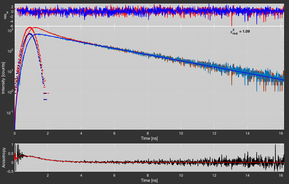
Fitting using an anisotropy model.
When using an anisotropy model, additionally the experimental and fitted anisotropy will be displayed below the main plot.
Extrapolation of the instrument response function
The experimentally determined instrument response function (IRF) might suffer noise due to low statistics, or be contaminated by a fluorescent impurity that comprises the ideal IRF pattern. In these cases, it is helpful to extrapolate the IRF using an appropriate model function. That model function is usually a gamma distribution, which is given by:
Here, the gamma distribution is given in the shape-rate parametrization with shape \(\alpha\) and rate \(\beta\), \(\Gamma(\alpha)\) is the complete gamma function, and \(s\) and \(b\) are parameters accounting for the shift of the IRF pattern and constant background.
The IRF pattern can be fit to the outlined model before the reconvolution fitting procedure is performed. Enable this option in the Settings tab by checking the Clean up IRF by fitting to Gamma distribution checkbox. The plot below the checkbox is used to show the result of the fitting procedure, whereby the measured IRF pattern is shown as blue dots, and the fitted model is given as a red line. The IRF pattern will automatically be fit to the model when the fit is started using the Perform reconvolution fit button.
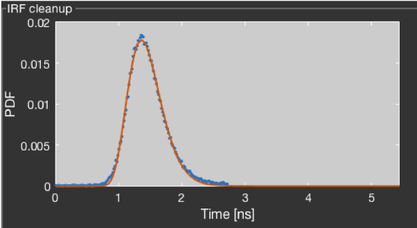
Extrapolation of the IRF using the Gamma distribution.
Simulation of \(\kappa^2\) distributions
When loading species-wise fluorescence decay data from BurstBrowser, additional functionality is available to determine the distribution of \(\kappa^2\) values from the available fundamental anisotropies of the donor and acceptor, as well as residual anisotropies of donor, acceptor, and FRET sensitized acceptor emission [Ivanov2009]. The program reports the average value with standard deviation. Additionally, the accuracy of determined distances (i.e. the deviation from the true distance value if \(\kappa^2 = 2/3\) was assumed) and the precision (i.e. the statistical uncertainty of the determined distance) is reported.
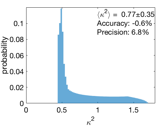
Simulated \(\kappa^2\) distribution using \(r_0(D)=0.4\), \(r_0(A)=0.4\), \(r_\infty(D)=0.1\), \(r_\infty(A)=0.1\) and \(r_\infty(DA)=0.05\).
Additional settings and exporting
- Use weighted residuals:
Tail fitting and reconvolution fitting support the use of weighted residuals. If Use weighted residuals is unchecked, the fit quality will be judged based on the mean squared deviation only.
\[\textrm{Mean squared deviation} = \frac{1}{N-P-1}\sum_i (x_i-f_i)^2\]Here, \(x_i\) are the data points, \(f_i\) is the model function, \(N\) is the number of data points and \(P\) is the number of fit parameters (i.e. \(N-P-1\) is the number of degrees of freedom). If Use weighted residuals is checked, the error for each data point \(\sigma_i\) will be estimate assuming Poissonian counting statistics, i.e. \(\sigma_i = \sqrt{x_i}\). The reduced chi-squared value \(\chi^2_{\textrm{red.}}\) is the maximum likelihood estimate for Gaussian errors and is defined by:
\[\chi^2_{\textrm{red.}} = \frac{1}{N-P-1}\sum_i \frac{(x_i-f_i)^2}{\sigma_i^2}\]\(\chi^2_{\textrm{red.}} \approx 1\) indicates a good fit, while \(\chi^2_{\textrm{red.}} >> 1\) means that the model is not sufficient to describe the data. \(\chi^2_{\textrm{red.}} < 1\) is an indication for overfitting, meaning that the complexity of the model should be reduced.
For anisotropy fitting, the usage of weighted residual is not available, since no straight-forward estimate is available for the estimation of the error of the calculated anisotropy.
- Automatic fit update:
- Automatic fitting can be enabled in the Setting tab by checking the Automatic fit checkbox. This will cause the fit to automatically update whenever sliders are changed.
- y-axis scale:
- The y-scaling of the main plot can be changed between linear and logarithmic by right clicking the main plot and selecting Y Logscale.
- x-axis scale:
- The x-scaling of the main plot can be changed between linear and logarithmic by right clicking the main plot and selecting X Logscale.
- Exporting plots:
- Plots can be exported by clicking Export Plot in the right-click menu, which will open the current plot in a new MATLAB figure.
- Exporting data:
- The fluorescence decay or anisotropy data can be exported as a .txt file by clicking Export -> Save Data to .txt. This will create a file with ending *_tau.txt or *_aniso.txt, depending on what kind of data is plotted. To compare exported data, click Export… -> Compare Data and select the exported .txt files. This will automatically create a comparison plot. When comparing fluorescence decays, the data will be aligned with respect to the maximum intensity point.
- Alternatively, the currently plotted data can be copied to the clipboard, so it can easily be pasted into other software like Excel or Origin (Export… -> Copy Data to Clipboard).
- TauFit integrates with the filtered-FCS functionality of PAM to generate synthetic microtime patterns. This is supported only when using an anisotropy model. Perform a fit and go to Export… -> Export fitted microtime pattern to export the current fit as .mi file that can be used in filtered-FCS analysis.
| [Koshioka1995] | Koshioka, M., Sasaki, K. & Masuhara, H. Time-Dependent Fluorescence Depolarization Analysis in Three-Dimensional Microspectroscopy. Applied Spectroscopy 1–5 (1995). |
| [Lakowicz2007] | Lakowicz, J. R. Principles of Fluorescence Spectroscopy. (Springer Science & Business Media, 2007), Chapter 4, Section 11. |
| [Ivanov2009] | Ivanov, V., Li, M. & Mizuuchi, K. Impact of emission anisotropy on fluorescence spectroscopy and FRET distance measurements. Biophys J 97, 922–929 (2009) |