Getting Started

Contents

• Getting Started
  • Installing PAM
    • Installing the stand-alone version of PAM
    • Installing and updating the open-source version of PAM
      • Downloading from the repository
      • Using Git
        • Installing Git
        • Downloading and updating using Git
      • Via MATLAB Git Integration
    • Modification and development of PAM
  • Where to find the sample data
  • Setting up PAM
    • Setting up a Profile
  • FCS and FCCS
    • Performing FCS calculations
    • Using FCSFit
  • Single-molecule FRET
    • Extracting bursts for single-molecule FRET
    • Using Burst Browser
  • Image Analysis
    • Exporting image data from PAM
    • Using MIA
      • Loading data into MIA
      • Performing image correlations in MIA
    • Using MIAFit
  • Phasor approach to FLIM
    • Calculating lifetime phasor data
    • Phasor Analysis

In this part, we try to give a brief step-by-step walkthrough for the installation and usage of the main functions of PAM and its sub-modules. In most cases, the walkthrough will be based on the example data provided at https://gitlab.com/PAM-PIE/PAM-sampledata. More advanced methods and settings are explained in other parts of the manual.

Installing PAM

The program can be downloaded from the homepage of Prof. Don C. Lamb - http://www.cup.uni-muenchen.de/pc/lamb/ - or through GitLab - https://gitlab.com/PAM-PIE.

This GitLab group contains four projects:

• PAM: The open-source version of PAM used with MATLAB.
• PAMcompiled: A compiled stand-alone version that does not require MATLAB.
• PAM-sampledata: Some example data the user can use to try out the PAM functionalities.
• PAMdocs: Project that contains files for the developers to update the PAM documentation and manual.

Installing the stand-alone version of PAM

1. Verify the correct MATLAB Runtime is installed (currently v9.1/ Matlab 2016b).

   You can download the MATLAB Runtime from the MathWorks Web site by navigating to

   http://www.mathworks.com/products/compiler/mcr/index.html

   For more information about the MATLAB Runtime and the MATLAB Runtime installer, see Package and Distribute in the MATLAB Compiler documentation in the MathWorks Documentation Center.

2. Download the compiled version of PAM for your Operating system (MacOS or WIN) from

   https://gitlab.com/PAM-PIE/PAMcompiled

3. Unpack the files.

4. Run the PAM.exe (Windows) or run_PAM.command (MacOS) to start the program. For MacOS, consult the readme.txt and how_to_create_shortcut.txt for additional information.

Installing and updating the open-source version of PAM

The open source version of PAM requires a valid licence for MATLAB (2014b or newer). Certain features further need access to tool boxes (curve fitting, image processing, optimization, statistics and machine learning, parallel computing) to work.

You can obtain and update PAM either through direct download from Gitlab, using the command line through Git, or by using the MATLAB Git integration.

Downloading from the repository

1. Download the open source version of PAM from https://gitlab.com/PAM-PIE/PAM
2. Unpack the files.
3. Start Matlab and navigate to the PAM folder.
4. Type PAM into the Matlab command line to start the program.
5. To update, simply download the newest version and overwrite your files.

Using Git

Installing Git

Updating of PAM requires the installation of Git.

• MacOS:

  MacOS has Git pre-installed since version 10.9. Try to run git from the terminal. If the command fails, you can download Git from https://git-scm.com.

• Windows:

  Download and install Git from https://git-for-windows.github.io.

Downloading and updating using Git

• To clone the repository, type git clone https://gitlab.com/PAM-PIE/PAM.git PAM to create a local copy of the repository in the folder PAM.

  • By default, you are checkout on the branch master, containing the stable version of PAM.
  • Should you need the newest updates, switch to the develop branch by typing git checkout develop.
  • To switch back, type git checkout master.

• To update, simply type git pull to obtain the newest changes. Note that this will only update the branch that you are currently on.

Via MATLAB Git Integration

To use all features of the MATLAB Git integration, it is recommended to install Git as described above.

1. Create a folder for PAM.
2. Start Matlab and navigate to the PAM folder.
3. Right click the ‘Current Folder’ panel in Matlab and select ‘Source Control’ and ‘Manage Files…’.
4. Set the ‘Source control integration’ to ‘Git’ and enter for the ‘Repository path’ https://gitlab.com/PAM-PIE/PAM.git.
5. Click ‘Retrieve’ to download the files automatically.
6. To update the PAM Git repository to the latest version, simply type !git pull into the MATLAB command line.

To update, you can alternatively use the MATLAB Git integration, however the !git pull method is easier and quicker.

1. Right click the ‘Current Folder’ panel in Matlab and select ‘Source Control’ and ‘Fetch’.
2. Right click the ‘Current Folder’ panel in Matlab and select ‘Source Control’ and ‘Manage Branches’.

3. Select the current branch form the remote repository, called ‘origin’.

   If you work on branch master, select origin/master (or refs/remotes/origin/master).

4. Click ‘Merge’ to merge the changes from the remote into you local repository.

Modification and development of PAM

Users are encouraged to modify the code of PAM for their individual needs and help with the development of new and the improvement of existing functionalities.

To report bugs or suggest improvements and bugfixes, please use the Issues function of GitLab. For this, a free GitLab account is required.

To contribute to PAM, please consult the contribution guide.

Where to find the sample data

The sample data is provided at https://gitlab.com/PAM-PIE/PAM-sampledata, including profiles for the different setups. Copy the profile files (.mat) into the /profiles folder of your PAM installation and restart PAM to make them available.

Setting up PAM

PAM is designed as a program running in the MATLAB environment. The used functionalities require a licensed MATLAB version 2014b or later and several toolboxes (optimization, statistics and imaging). A compiled standalone version that does not require a MATLAB installation will be available, but with limited functionalities especially for data export and custom plotting, since no access to the raw data is available via global variables. To install PAM, simply download the .zip file and extract it. Open MATLAB and navigate to the PAM folder. It is advised not to add the PAM folder to the Matlab path, as this might create confusion later on when using concurrent PAM versions. Here, type PAM into the command window to start PAM, or type the name of a sub-programs to start the particular window directly. Alternatively, right-click the respective .m file and select Run.

Setting up a Profile

All settings in PAM are defined in a user profile that can be selected in the Profiles list in the top-left corner of the Profiles tab in PAM. A minimal starting profile is automatically created, if none exists. How to create a new profile is described for the example of a two-color PIE microscope with individual detectors and B&H SPC150 TCSPC cards for green and red. The sample data is found in the /SetUp folder.

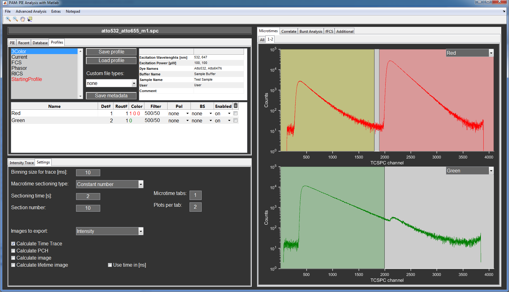
Overview of the Profile and Settings configured for the example explained below.

Right click the Profiles list and select Add new profile to create a new profile.

A popup will open asking for a name for the profile. Click Ok once you typed in the name.

Click on the new profile in the Profile list and press enter or right click and select Select profile.

The new profile now only has one detector channel. In our case, we need a second channel for the red detector.

Alternative 1: Right click on the Detector list and select Add new microtime channel. We now have to set the Det# value of the second channel to 2, corresponding to our second TCSPC card.

Alternative 2: PAM has an automatic channel detection feature. When data is loaded that is not associated with an existing channel, a new channel will be created automatically. To turn this feature off/on, right click the Detector list and select Auto-detect used detectors and routing

Load the data set atto532_atto655_m1.spc from the /SetUp folder using the Multi-card B&H SPC files recorded with B&H-Software routine.

You can change the color and name associated with the channels as you like (e.g. Green and Red).

To display the microtime histogram of both channels, we adjust the Microtime tabs and Plots per tab properties in the Settings tab. In this case, we set the Plots per tab to two. Now, the histograms are shown in the Microtimes tab.

Now, we need to define PIE channels. Most calculations and functions of PAM are based on these PIE channels.

Initially, a single PIE channel associated with the first detector channel is created. In our example, we need to create two more. For this, right click the PIE channel list and select PIE channel and Add new PIE channel.

For the two-color PIE setup, we need one PIE channel for the green detection after green excitation (GG), one for red detection after red excitation (RR) and a third for red detection after green excitation (GR). The last combination possible PIE channel of green detection after red excitation (RG) does not contain useful signal and can be neglected.

Set the associated detector channel of the GR and RR channels to the red detector and GG to the green.

The microtime ranges associated with each laser depend heavily on each individual setup. In this case we assume that the green laser pulse arrives in the first half of the microtime range and the red in the second half. The total range is 4096 TCSPC channels.

Set the range for the GG and GR channels to 1-2048 and the RR channel to 2049-4096.

You can also change the color associated with each channel by right clicking the PIE channel list and selecting PIE channel -> Change channel color, or via the c key.

The different PIE channels should now also be indicated in the microtime histograms as colored backgrounds. Make sure that they overlap with the corresponding decays.

FCS and FCCS

Performing FCS calculations

To perform FCS and FCCS calculations, first load your data. You can also load multiple files at once. The data will then be concatenated and treated as a single, longer measurement.

In this case, we will show how to perform correlations based on the atto532_atto655 B&H .spc example data. For this, select the FRET-FCS profile. Here, we have a total of 4 detectors, for green parallel, green perpendicular, red parallel and red perpendicular.

First load the data. For this, you need to select the _m1.spc format (B&H multi-card format).

To select on which particular PIE channels you want to perform the auto- and cross-correlation, use the checkbox table in the Correlate tab. The diagonal elements represent the auto-correlations. The others correspond to the cross-correlation of the row and the column PIE channels.

For this example, we will calculate the auto-correlation for the green and the red channels plus the cross-correlation between them.

For the auto-correlations we will correlate GG1 with GG2 and RR1 with RR2. By calculating the correlation from signal of two different detectors and TCSPC cards, we can remove correlation artifacts from detector afterpulsing and TCSPC dead time. This is especially noticeable at very short delay times (~100ns). Since the dyes are freely rotating, any polarization effects can be neglected in this case.

For the cross-correlation, we will use the combined channels to improve the photon statistics. For green, this is the GG1+GG2 PIE channel. For red, we will use the RR1+RR2 channel. We can also do a cross-correlation between the green channel and the full red channel (GR1+GR2+RR1+RR2). This represents the case of not using PIE.

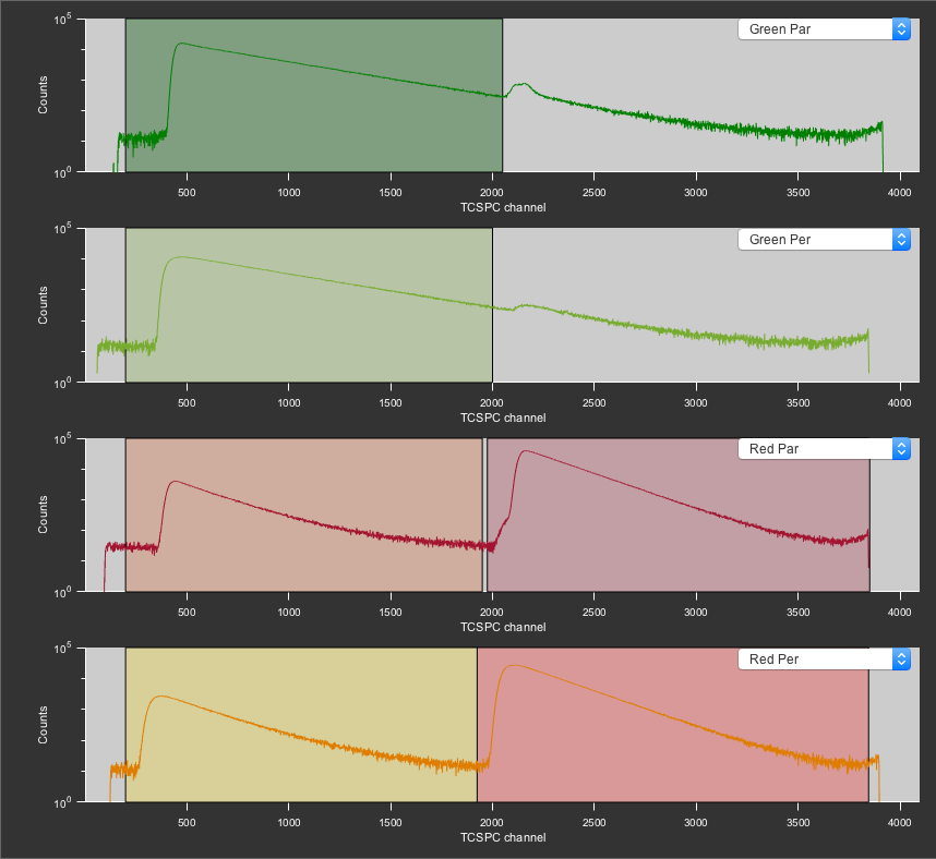
The PIE channels defined for the FCS measurement. Top to bottom: GG1, GG2, GR1 and RR1, GR2 and RR2.

Next, select the type of correlation (for standard FCS use Point) and the file type. The .mcor format is a PAM specific type based on the standard Matlab data format (.mat) and can be easily loaded into Matlab (for plotting etc.). The .cor format is a simple text file that can be used to look at the data outside of Matlab or PAM. Both can be analyzed with the FCSFit sub-module.

FCS calculations are done in individual segments, indicated by the gray segments in the intensity trace plot. You can set either the total number of segments or their length with the Section time or the Section number properties in the Settings tab.

You can remove individual segments from the calculations by simply left clicking on them. This is useful to remove small artifacts, like aggregates, air-bubbles or dust, from the correlation.

To start the correlation, simply press the Correlate button in the Correlate tab. The files are saved automatically in the folder of the raw data with the same filename and an added suffix of ‘channelname1_x_channelname2’.

Once the calculation is finished, the correlation curves will be shown in the bottom right plot. Each selected PIE channel combination is displayed in an individual plot. The individual curves represent the selected segments. They can be discarded individually with a left click on the curves. If you choose to unselect segments at this point, right click the plot and select Save selected correlations to update the file to you new selection.

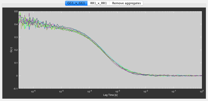
The preview plot of the individual segments after the correlation has been performed.

Multiple files can be correlated separately by clicking the Multiple button in the Correlate tab. A file selection dialog will open and the user can select multiple file to be correlated. Each selected file is loaded and correlated separately one after another. The same settings (PIE channels, selected segments, etc.) are used for all of them.

Another way to automatically perform multiple correlations is done using the database functions.

Using FCSFit

FCSFit is the sub-module of PAM for analyzing FCS and FCCS data. It can be opened via the Advanced Analysis menu in the menu bar of PAM or from the command window by typing in FCSFit.

Here we will show its functions on the case of the data used for the FCS part (atto532_atto655).

Once you opened the window, first load the fit model you want to use. Select File and Load Fit Function. The last fit model used during the previous session will be preloaded. For this example, load the FCS_TauD.txt model. This is a simple diffusion through a 3D gaussian focus model with an added triplet dynamics term.

Next, load the correlation files. File -> Add Files will add the new files to previously loaded once, while Load New Files will clear the previous entries.

The fit parameters can be adjusted in the Fit parameters table in the Fit tab at the bottom. The F anf G checkboxes can be used to fix or globally link individual parameters, respectively.

The settings for the fitting procedure can be adjusted in the Settings tab.

Select Start…Fit in the menu bar to begin the fit.

Once the fit is finished, the results will be displayed in the Fit parameters table.

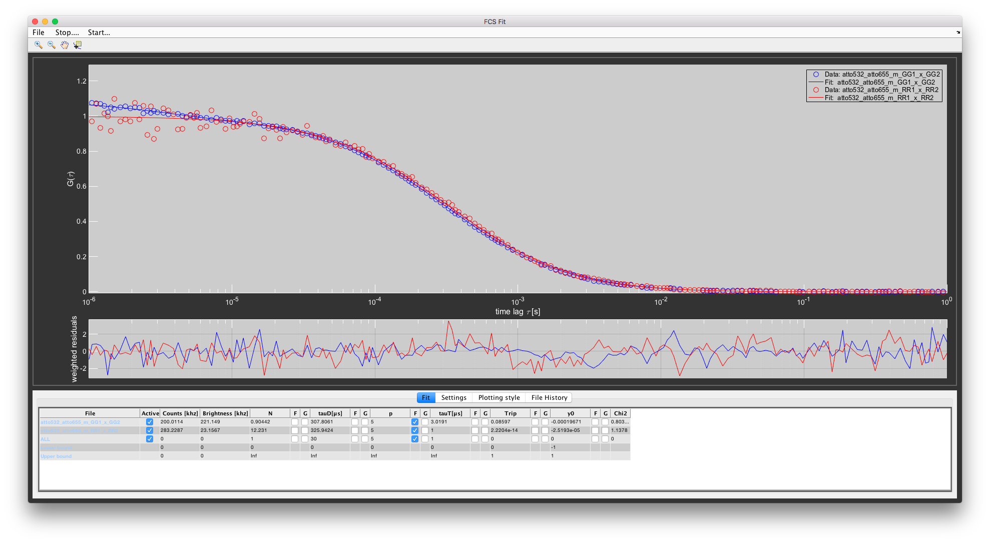
Fits to the autocorrelation functions GG1xGG2 and RR1xRR2.

The fit results can be copied to the clipboard with the Copy Results to Clipboard options accessed by right-clicking the Fit parameters table.

The FCS curves and fits can also be exported to a new Matlab figure with a right click on the plot and selecting Export to figure. The export settings can also found in the Settings tab.

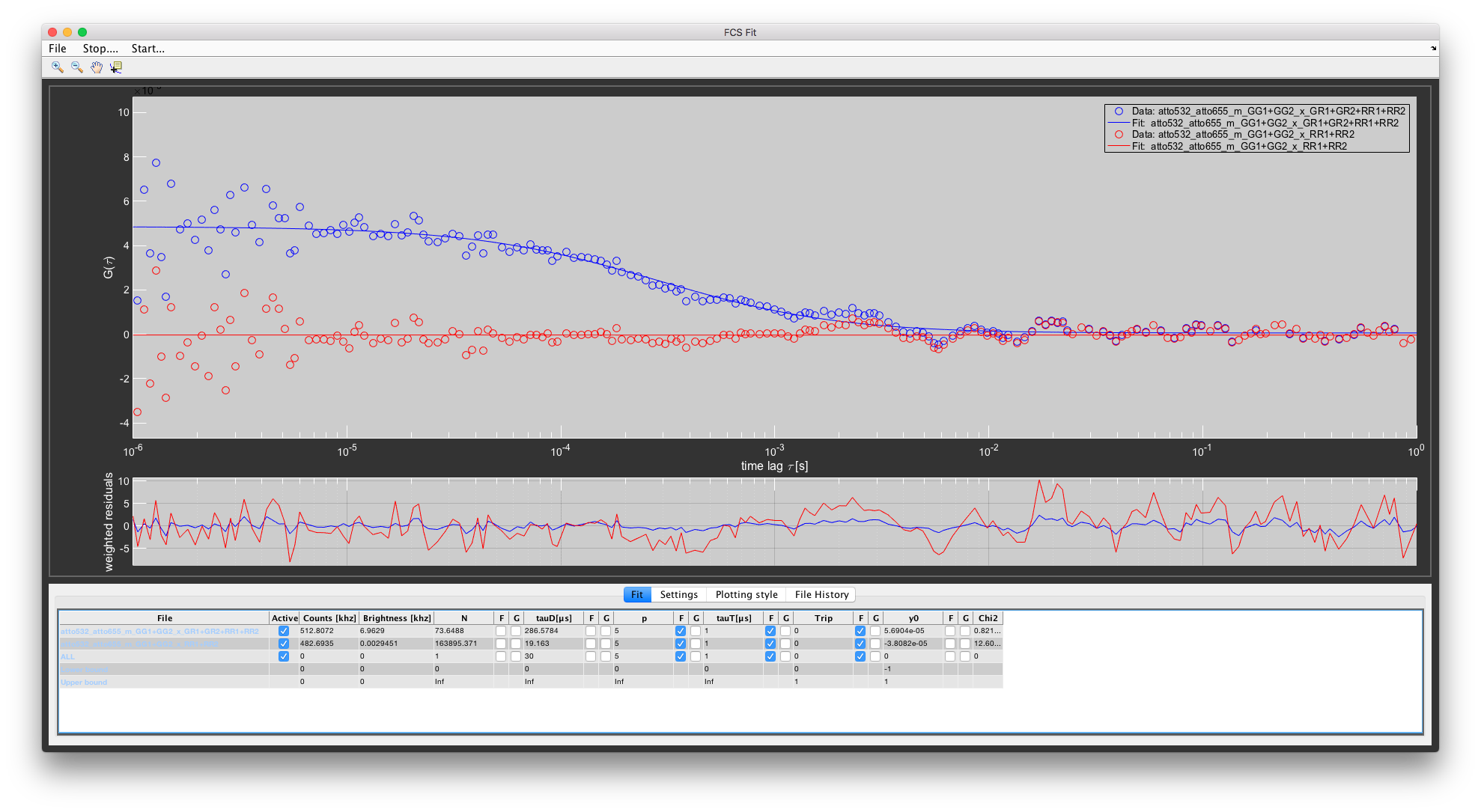
Fits to the cross-correlation functions (GG1+GG2)x(RR1+RR2) - i.e. using PIE, and (GG1+GG2)x(GR1+GR2+RR1+RR2) - i.e. not using PIE. When PIE is not used, the spectral cross-talk of the green dye leads to residual cross-correlation amplitude.

Single-molecule FRET

For this tutorial, use the FRET-FCS-profile and load the sample data DNA_1h using the option Multi-card B&H SPC files recorded with B&H-Software. The data folder additionally contains measurements of the buffer and a pure water sample to measure the instrument response function (IRF) for lifetime fitting. The profile already contains the data from these measurements (background photon counts, IRF pattern), so we do not need to load these data files here. See the section in the PAM manual for a description of how to define these calibrations.

Extracting bursts for single-molecule FRET

The loaded data was recorded using PIE and polarized detection, resulting in for detection channels and a total of 6 PIE channels (GG1, GG2, GR1, GR2, RR1, RR2), which are already set up in the profile.

Switch to the Burst Analysis module in PAM. Select Sliding Time Window as Smoothing Method and APBS 2C-MFD as the Burst Search Method. This will perform an all-photon burst search (APBS), pooling all photons of the individual detection channels into one, using the sliding time window burst search. First, we need to assign PIE channels to the FRET channels used in the burst analysis. FRET channels are denoted by DD for the donor signal after donor excitation, DA for the FRET signal after donor excitation, and AA for the acceptor signal after direct excitation by the acceptor laser, split into parallel and perpendicular polarization. Assign the PIE channel GG1 to DD-parallel, GG2 to DD-perpendicular, GR1 to DA-parallel, GR2 to DA-perpendicular, RR1 to AA-parallel and RR2 to AA-perpendicular. Now, set the burst search parameters as 500 \(\mu\) s for the time window, 100 photons minimum per burst and a threshold of 5 photons per time window (i.e. 10 kHz count rate threshold).

Click the Preview button to see a preview of the burst search. Use the arrow to navigate through the preview plot.

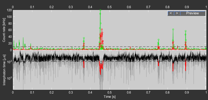
Preview of the burst search.

Press the Do Burst Search button to start the burst search. This will perform the burst search and store the result in a .bur file using the filename of the raw data in a sub-folder with the name of the raw data. After the burst search has been performed, the Do Burst Search button will be green. For a description of how to determine the burstwise fluorescence lifetime and the two channel kernel density estimation filter (2CDE), see the respective section in the PAM manual.

Using Burst Browser

Open BurstBrowser using the menu Advanced Analysis -> BurstBrowser or by typing BurstBrowser in the command-line. Click File -> Load New Burst Data and select the file DNA_1h_m1_APBS_2CMFD.bur in the DNA_1h_m1 subfolder.

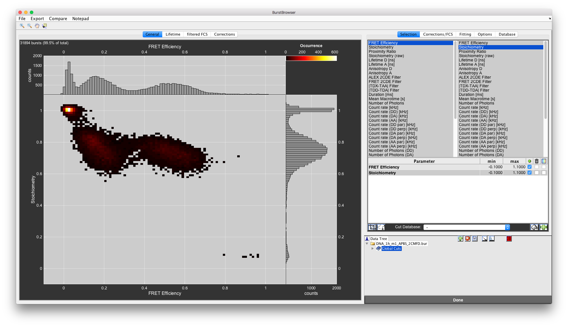
The unprocessed burst analysis result shows two FRET populations.

You can change the plotted parameters using the lists in the top right. The left list selects the parameter for the x-axis, the right parameter for the y-axis. Right-click any parameter to add it to the Cut Table, where you can specify lower and upper bounds to constrain the data selection.

In this case, we want to exclude the donor-only and acceptor-only populations. To do so, set restrict the range for the Stoichiometry in the Cut Table to the interval [0.3,0.9]. This will remove contributions of donor- and acceptor-only molecules to the FRET efficiency histogram completely.

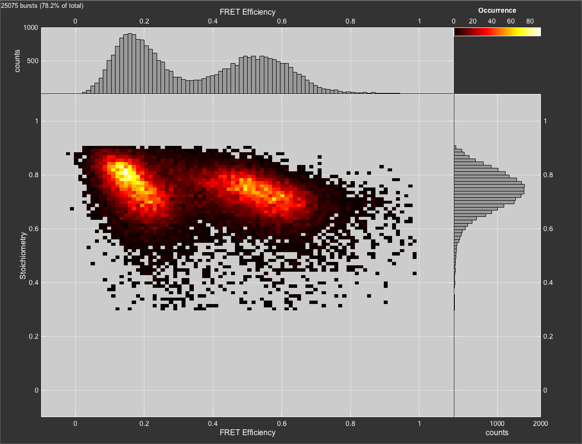
Filtered burst data after removal of donor- and acceptor-only molecules through the stoichiometry parameter.

For a more detailed description of the functionalities of BurstBrowser see the manual.

Image Analysis

The key steps of using the image analysis functions of PAM will be explained with the example of the RICS_EGPF.ppf file. For this, select the RICS profile first.

Exporting image data from PAM

There are two ways to export the image data of the individual PIE channels from PAM.

The first one is to load the data into PAM.

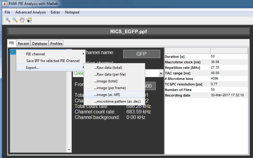
Next, select the PIE channels in the PIE channel list for which you want to export the data.

Right click the list and select Export.. and ..image (as .tiff).

Select the folder in which you want the new image files to be saved.

For each selected PIE channel a separate file will be created with the raw data file name and the PIE channel name as a suffix.

The second way of exporting TIFFs from PAM uses the database functions and is explained here.

Exporting images as TIFF stacks.

Using MIA

MIA is the image analysis module of PAM. It can be started from PAM via Advanced Analysis or from the command line by typing in Mia.

Loading data into MIA

MIA can use two types of data.

The first uses the image data currently loaded in PAM.

To load this data, use the Load… and …data from PAM functions in MIA. The PIE channels used for this are defined in the Channels tab with the PIE Channels to load options.

The more common type of data is based of TIFFs. Generally, MIA can use any type of data that can be converted to TIFFs, either with PAM (explained above) or other programs.

To load new TIFFs, use the Load… and single color TIFFs functions in MIA.

Next, select your desired TIFF files for the first channel and click Open. When multiple files are selected, they will be simply concatenated.

A new file selection will open up, asking you to select the files for the second channel. Click Cancel if you only want to analyze single color/channel data.

The data will them be loaded and displayed.

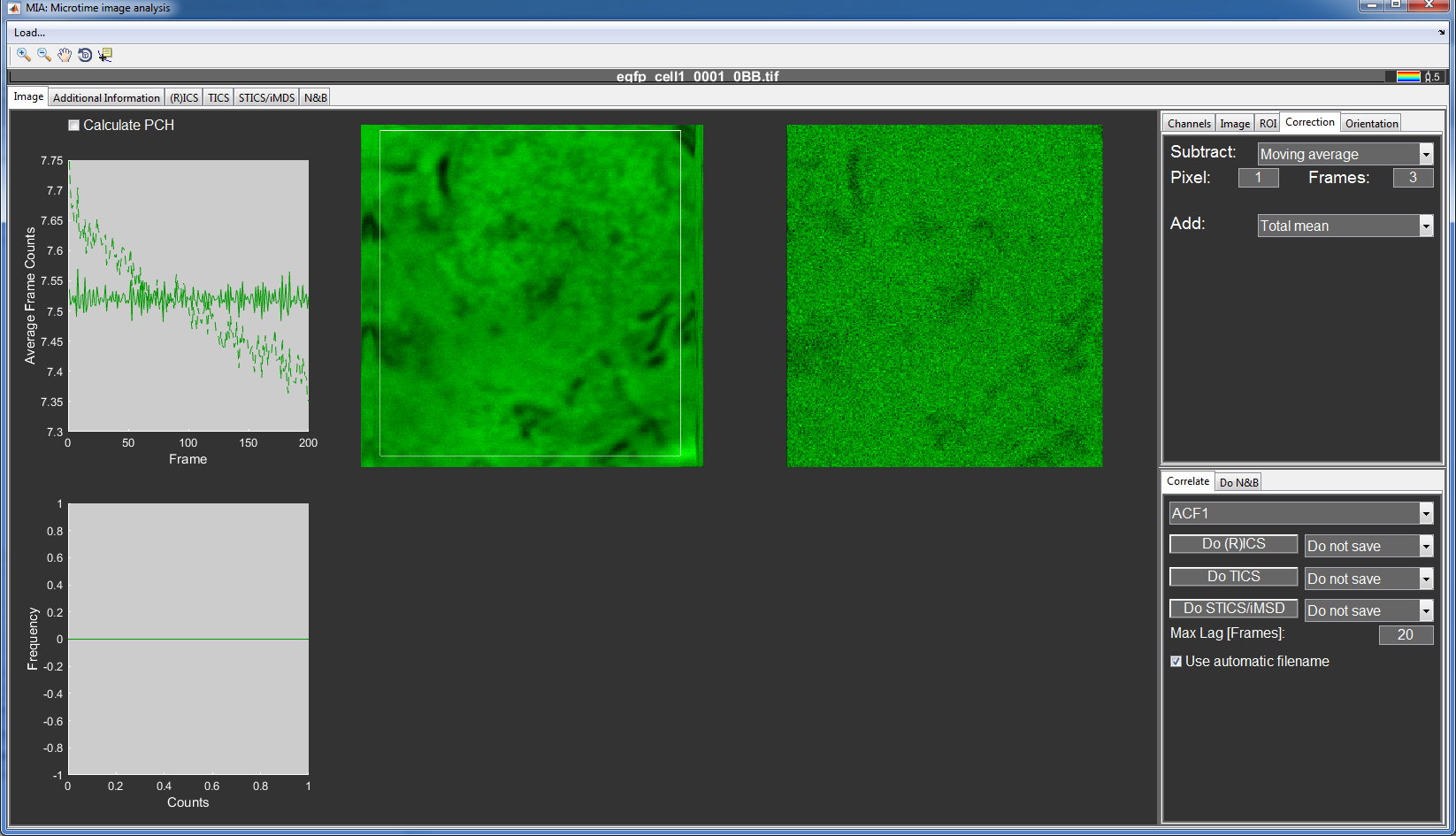
Single color data loaded into MIA.

Performing image correlations in MIA

To do any type of analysis in MIA, fist load the data.

Select a subregion of the loaded file in the left image plots of MIA. This can be done with the mouse in the left images or with the edit boxes in the ROI tab.

An advanced region of interest selection can be employed by selecting the Arbitrary region ICS settings in the ROI tab.

The images can then be further adjusted in the Correction tab. This can be useful, e.g. to remove immobile structures for RICS analysis or bleaching effects for TICS.

For the RICS_EGFP data, select a moving average of 1 Pixel and 3 Frames to be subtracted and add the total mean to keep the mean intensity constant.

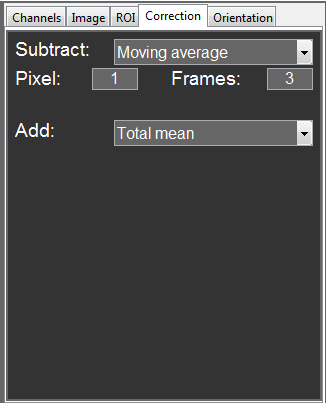
Standard correction settings for RICS analysis.

This removes the correlation from immobile structures in the cell and also corrects for the slight bleaching.

Now that the images are corrected, you can calculate the image correlation by pressing the Do (R)ICS button.

To save the data, choose a file format before performing the correlation. .miacor is a format based on the Matlab data format and can easily be loaded into the MATLAB workspace at a later point in time. You can also save the data as TIFFs to look at them with other image analysis programs. Both file formats can be loaded into MIAFit.

With the standard settings, the program creates a MIA folder in the folder of the raw data and saved the correlation files automatically. For the filename, the program used the original name with a suffix for the correlation channel (ACF1, ACF2 or CCF). Additionally, a info file is generated that contains the key settings used.

You can activate a manual file naming by unselecting the Use automatic filename checkbox.

You can have a quick look at the correlations in the (R)ICS tab, but the main way of analysis is performed with the sub-module MIAFit.

Using MIAFit

MIAFit can be started from the Advanced Analysis menu in PAM or by typing MIAFit into the matlab command line.

MIAFit works basically the same as Using FCSFit.

The difference is in the way the 2D data is displayed.

You can switch between on-axis view for all files (On-Axis tab) or a full 2D correlation display for a single file (2D Plots);

For the RICS_EGFP file, load the RICS_Simple3D model. Set the pixel size (Px) to 40 nm, the pixel time (P_time) to 11.11 \(\mu s\) and the line time (L_time) to 3.33 ms and fix all these values. It is generally useful to fix the axial focus size (w_z), because this parameter is often hard to determine with RICS. Set it to 1 \(\mu m\).

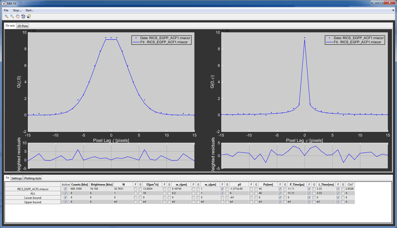
MIAFit RICS analysis window.

Phasor approach to FLIM

Calculating lifetime phasor data

How to calculate phasor data from you raw data file is explained for the example of the sample phasor data provided with the download. The data is based on the PAM simulation file format.

First, switch to the Phasor profile. This profile is configured for a single detector channel and a single PIE channel.

Load a reference file (Phasor_Reference_4ns.sim). Remember that you have to select the PAM simulation file (.sim) format in the file selection menu.

Go to the Phasor Referencing tab in the Additional tab.

Since this example only has one channel, the correct channel is already selected. In other cases you might have to first select the correct detector channel from the dropdown menu. Phasor referencing works directly on the detector channels and is independent of the PIE channels

Define the loaded file as the reference by clicking the Use MI as reference button. Now, this microtime histogram will be used as the reference file until it is replaced, even across sessions.

Next, load the files you want to use (Phasor_Sample.sim) for the phasor calculations.

Use the Range to use fields to adjust the microtime range used for the calculation to your data. For example, if you recorded two color PIE data and want to analyze the red lifetime, remove the green cross-talk or FRET part from the range. The program uses the full microtime range, but sets all values outside of the defined range to zero. In this case you can use the full range of 1-8192.

Before performing the calculation, set the Ref LT field to the lifetime of your reference (here 4ns) and the TAC field to the duration of the full microtime range (here 40ns).

To calculate the phasor and save the data, click the Calculate Phasor Data button. Select a path and filename and click Save to save the data.

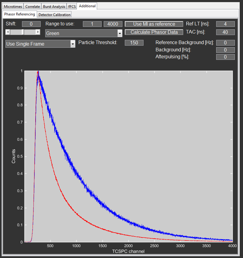
Phasor Referencing setup for the provided sample data.

Phasor Analysis

The main features of the phasor analysis sub-module are explained for the example of the sample phasor data provided with the download.

Open the Phasor analysis window from the Advanced Analysis menu in PAM or by typing in Phasor into the MATLAB command line.

Use Load Phasor Data to load files you created with PAM or the one provided with the download (Phasor_Reference_4ns.phr and Phasor_Sample.phr).

The intensity images are now shown to the nine image plots at the left hand side of the window. The files are also added to the Phasor file list in the bottom right and the phasor histogram is plotted in the top right.

You can (de)activate individual files by selecting them in the Phasor file list and using with the arrow keys or remove them with the del key. The + key will set the file to inactive, meaning that it will be used for calculating the phasor histogram, but not shown in the image plots.

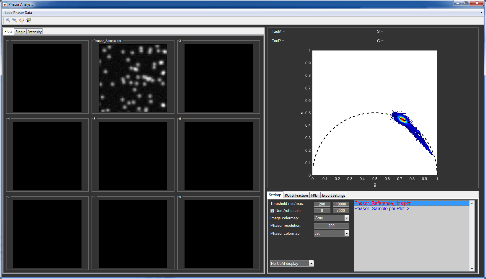
Phasor analysis window of the provided sample data. The first file in the list is shown in red, meaning that it is in the inactive state.

The threshold values remove pixels with intensity below or above the set values from the phasor histogram. You can change them to see how it affects the histogram.

The other parameters in the Settings tab mainly affect how the data is displayed.

In order to indicate the phasor position in the images, there are two principle ways:

Method 1: Region of interest.

Press and hold the number keys 1-6 and click into the phasor histogram to select a region of interest. The left mouse button creates a rectangular and the right mouse button a ellipsoid ROI.

The pixels inside this ROI will now be assigned the color associated with the corresponding ROI

You can change the width of the ellipsoid and the color in the ROI&Fraction tab.

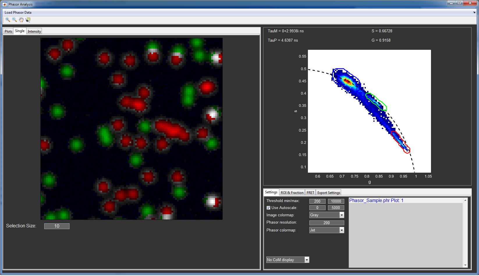
ROI selection for Phasor analysis

Method 2: Position indication.

Press and hold the number keys 0 and click into the phasor histogram to place a line into the phasor histogram.

The pixels will be assigned a color corresponding to the closes point on this line.

You can change the maximal distance from the line and the color-code use in the ROI&Fraction tab.

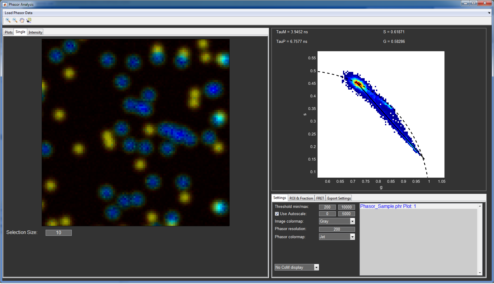
Line selection for Phasor analysis

Use the mouse wheel to zoom into the phasor histogram and the left mouse button to move the view.

Right click the images to export them.

Double click the phasor histogram to export it to a new figure. The setting for this can be adjusted in the Export Settings tab.